3D animation of regional cross-sections for high-resolution climate data

Motivation

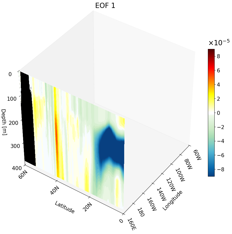
In the previous tutorial I taught you how to create 3D visualizations for zonal, meridional, and depth cross-sections. Though the cross-sections are great, sometimes they are hard to understand and intuitively place their location. For example, the meridional cut is tough to understand on its own:

Meridional Cross

Meridional cross-section at 160E in the North Pacific. This is harder to place intuitively than the cube.

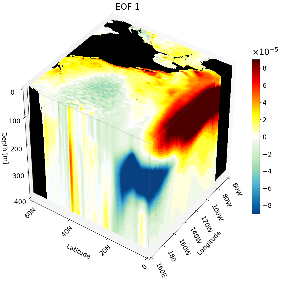
But if you visualize this cut with other cross-sections we can better interpret the figure.

Cube

North Pacific with a depth, zonal, and meridional cross-section.

You can also plot multiple of the same cross-sections at once. This is great for publications to show how the climate changes with depth, latitude, or longitude.

multi zonal

Multiple zonal cross-sections for the California coast.

I’ve found animating the cross-section has more impact, especially for presentations.

In this tutorial we will go over how to create an animation of cross-sections by using functions created in the previous tutorial. You can find the full code in this repo.

Background and Set Up

For information on the data please see the data and methods section of this post. The main thing you need to keep in mind is we are working with high-resolution data ($1/12^{\circ}$ latitude by $1/12^{\circ}$ longitude with 50 depth layers). This means that regional animations are going to look great! We will be taking advantage of this and mostly animating within the Pacific region.

Here are the libraries you will need:

# all visualization libraries
import matplotlib as mpl
import matplotlib.pyplot as plt
from mpl_toolkits.mplot3d import Axes3D
from matplotlib import cm
from matplotlib.colors import ListedColormap, LinearSegmentedColormap

# to get path
import os

# libraries to read data
import netCDF4 as nc
from netCDF4 import Dataset as ds
import numpy as np

# libraries used for some math
from numpy import linspace
from numpy import meshgrid
import math

For the climate data I build a custom colormap:

# Creating the custom colorbar
top2 = cm.get_cmap('GnBu_r')   # get green blue colormap
bottom2 = cm.get_cmap('hot_r') # get hot colormap
top_array = top2(np.linspace(0, 1, 128))        # create array with color values
bottom_array = bottom2(np.linspace(0, .9, 128)) # create array with color values
# edit array with color values to have better transition shades
top_array[-2:,:] = bottom_array[0,:]
top_array[-3,:] = np.array([1., 0.98823529, 1., 1.])
top_array[-4,:] = np.array([0.96862745, 0.98823529, 1., 1.])
top_array[-5,:] = np.array([0.96862745, 0.98823529, 0.94117647, 1.])

newcolors2 = np.vstack((top_array, bottom_array))         # stacking color arrays on top of each other
newcmp2 = ListedColormap(newcolors2, name='OrangeBlue')   # creating new colormap

To format the latitude and longitude axes I use two main functions that will add N (north) or S (south) to the latitudes and W (west) or E (east) to the corresponding longitudes.

#################################################################################################################
#################################################################################################################
# Function formats longitude to get rid of degree symbols
# Input:
#         - longitude: int with longitude from 0 to 360
# Output:
#         - string with longitude value and W (west) or E (east)
def format_longitude(longitude):
    if not 0 <= longitude <= 360:
        return "Invalid longitude. Must be between 0 and 360 degrees."

    if longitude == 0:
        hemisphere = ''
        degrees = longitude
    elif longitude < 180:
        hemisphere = 'E'
        degrees = longitude
    elif longitude == 180:
        hemisphere = ''
        degrees = longitude
    else:
        hemisphere = 'W'
        degrees = 360 - longitude

    return f"{degrees:.0f}{hemisphere}"

#################################################################################################################
#################################################################################################################

# Function formats latitude to get rid of degree symbols
# Input:
#         - latitude: int with latitude in degrees. Positive values are N and negative are S.
# Output:
#         - string with absolute value of latitude and S or N
def format_latitude(latitude):
    if not -90 <= latitude <= 90:
        return "Invalid latitude. Must be between -90 and 90 degrees."
# adding S or N based on negative or positive value
    if latitude > 0:
        hemisphere = "N"
    elif latitude == 0:
        hemisphere = ""
    else:
        hemisphere = 'S'

    degrees = abs(latitude)

    return f"{degrees:.0f}{hemisphere}"

There are three functions used to process the data:

get_var: Used to read in the latitude, longitude, and depth variables of the data we are plotting. This is heavily dependent on the names of the variables in the data file.
vol_weight: Used to calculate the volume at each grid point. This is important to represent the dimensions correctly in the data, but is not necessary for plotting. The EOF is weighted, meaning the volume is already multiplied in; this means we need to divide the volume out for visualization.
read_EOFs: This reads in the data file and divides out the volume at the end.

#################################################################################################################
#################################################################################################################
# Function get_var() will get variables that will be required for EOFs
# Input:
#         - fn: a string with the complete path of the data
# Output:
#         - lat: 1D array with all latitude values
#         - lon: 1D array with all longitude values
#         - depth: 1D array with all depth values
#         - years: 1D array with all year values
# NOTE: Change variable names according to your file
def get_var(fn):
    fn     =  ds(fn,'r')
    lat    = fn.variables['lat'][:].data    # read in latitude
    lon    = fn.variables['lon'][:].data    # read in longitude
    depths = fn.variables['depth'][:].data  # read in depth
    fn.close()
    return lat, lon, depths
#################################################################################################################
#################################################################################################################
# Function computes volume weights based on latitude and depth values. Although longitude values are not
# in the equation, the length of the longitude array is necessary for building the 3D volume weight array.
# Input:
#         - lat: 1D array with all latitude values
#         - lon: 1D array with all longitude values
#         - depth: 1D array with all depth values
# Output:
#         - area_weight: 3D array with volume weight
def vol_weight(depths, lon, lat):
    xx, yy = meshgrid(lon, lat)
    tot_depth = len(depths)
    # area weight for latitude values
    area_w = np.cos(yy*math.pi/180)
    if lat[-1] == 90.0:
        area_w[-1,:] = 0.0
    # volume weights for depth
    volume_weight = []
    for i in range(tot_depth):
        if i == 0:
            volume_weight.append(np.sqrt(depths[0] * area_w)) # first depth thickness
        else:
            volume_weight.append( np.sqrt((depths[i] - depths[i - 1]) * area_w))
    # Turning weights into one array
    volume_weight = np.array(volume_weight)
    return volume_weight
#################################################################################################################
#################################################################################################################
# Function will read one EOF mode
# Input:
#         - mode: (int) describing which mode to read
# Output:
#         - EOF: 3D float array with the EOF at a defined cut
def read_EOFs(fn):
  get_var(fn)
  EOF_ncfile = ds(fn, 'r')
  EOF = EOF_ncfile.variables['EOF']
  EOF = EOF[:].filled()
  EOF_ncfile.close()
  volume_weight = vol_weight(depths, lon, lat)
  EOF = EOF/volume_weight  # remember to divide by volume weight
  return EOF

To read in the EOFs, just use os to change to the appropriate directory and then run:

# define the complete path with the file name
data_directory = os.getcwd()
fn     = 'EOF_1.nc'
fn     = os.path.join(data_directory, fn)

lat, lon, depths = get_var(fn) # read variables
EOF1 = read_EOFs(fn) # read EOF 1

Some Notes Before We Get Into Plotting Each Cross-Section

There is one main function that does most of the plotting. You can find the documentation for the function at https://matplotlib.org/stable/gallery/mplot3d/box3d.html.

For each of these plots, assume:

X-axis is longitude
Y-axis is latitude
Z-axis is depth

We define the variables X, Y, and Z as 3D arrays with their respective values, cut down to a specific range. To do this we use the meshgrid function with the order longitude, latitude, and depth. The meshgrid is built from cut dimensions to focus on a specific region.

The Overview

For each cross-section we create a function that will produce a figure object with one cut plotted. We will then save this figure as a PNG and put all the PNG files together into a GIF.

There are a few things that we keep separate from the function so that it is easier to customize the GIF without having to change the function:

The set up for the region
Defining the ticks for each axis
- This makes sure your labels aren’t too close together or too far apart
Defining the cross-sections you want to plot based on the indices
Setting up the bounds and total color bins for the colorbar
Creating the title

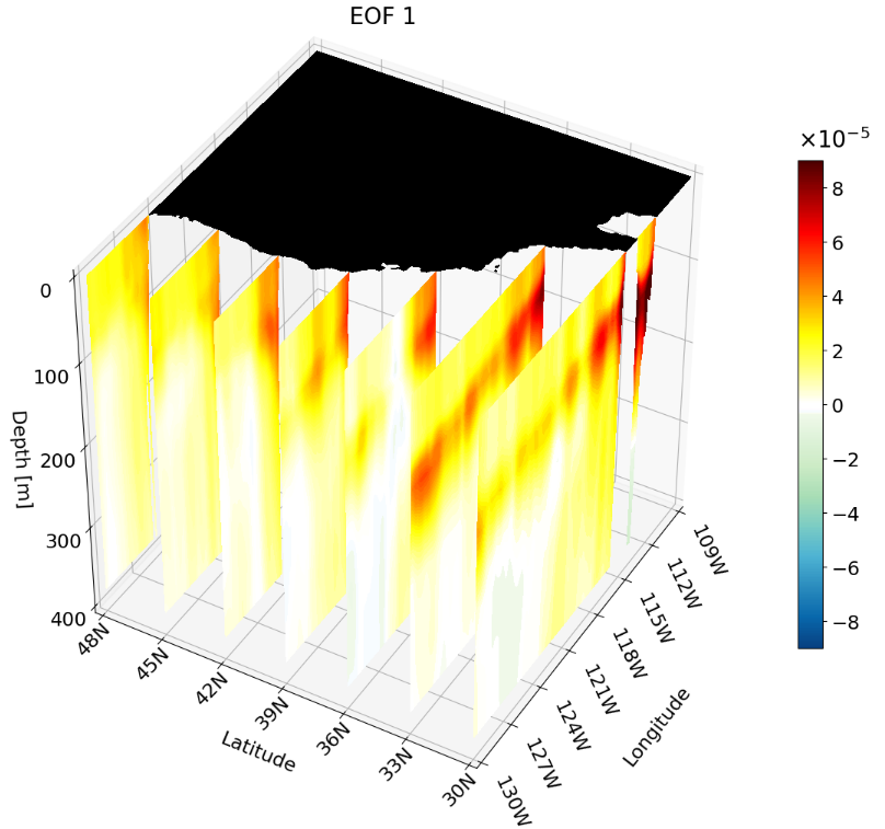
Zonal Cross-Section Animation

Let’s start with one of my favorite cross-sections: the zonal cross-section. This cut will tell us how the climate changes with latitude.

We will use the California coast as an example. We define the indices, tick labels, and the aforementioned meshgrid variables for this region:

# Set up cube for the California coast
lat_cut_start = 1320   # index for 30 N
lat_cut_end = 1537     # index for 48 N
lon_cut_start = 2760   # index for 130 W
lon_cut_end = 3013     # index for 109 W
depth_cut_end = 30     # index for 400

# Defining the range and position of each tick for labeling
# last number changes the interval
lon_ticks   = np.arange(lon[lon_cut_start], lon[lon_cut_end], 3)
lat_ticks   = np.arange(lat[lat_cut_start], lat[lat_cut_end], 3)
depth_ticks = np.arange(0, depths[depth_cut_end], 100) # if plotting the first 100 meters change the last number to something =<25

# create grid for each lat, lon, and depth variable
X, Y, Z = np.meshgrid(lon[lon_cut_start:lon_cut_end], lat[lat_cut_start:lat_cut_end], -depths[0:depth_cut_end])

We create a function that takes in the following arguments:

title: string with the title for each figure
EOF: 3D array with data to be visualized
clip: float clip value that defines the maximum and minimum for the colorbar
levels: int that sets how many colors you want to plot
lat_ind: int with the latitude index that defines the cross-section

The function can be broken down into 6 parts:

Figure object creation and set up
Land plotting for base map
Cross-section plotting
Axis labeling and formatting
3D view setting
Colorbar labeling and formatting

#############################################################################
#############################################################################
# Function will plot one zonal cross-section for a region
# Input
#         - title: string with title for each figure
#         - data: 3D array with data to be visualized
#         - clip: float clip value that defines maximum and minimum for the colorbar
#         - lat_ind: int with the latitude index that defines the cross-section
#         - levels: int that sets how many colors you want to plot
# Output
#         - fig: matplotlib figure object with the 3D figure
# Important variables
#         - lon_cut_start: int with starting longitude index
#         - lon_cut_end: int with end longitude index
#         - depth_cut_end: int with end depth index
# Note: make sure all tick values are defined before calling this function. This is
#       important for accurate labeling
#############################################################################
#############################################################################
def plot_zonal_3D(title, EOF, clip, levels, lat_ind):
    # --- Setup Figure ---
    fig = plt.figure(figsize=(12, 13))
    fig.subplots_adjust(right = .95)  # Add this line
    
    title_sz = 20
    label_sz = title_sz-3
    
    ax = fig.add_subplot(111, projection='3d')  # This is what defines the plot as 3D
    levels = np.linspace(-clip, clip, levels + 1) # sets ticks on colorbar
    
    # Contour Norms
    norm = mpl.colors.Normalize(vmin= -clip, vmax=clip)
    #############################################################################
    # plotting land
    surface3D = EOF[0, lat_cut_start:lat_cut_end,lon_cut_start:lon_cut_end]
    
    mask = np.isnan(surface3D) # create a mask for the NaN values
    masked_array = np.where(mask, surface3D, np.nan)          # change points with values to NaN
    masked_array = np.where(~mask, masked_array, -clip) # change NaN points to values
    _ = ax.contourf(X[:, :, 0], Y[:, :, 0], masked_array, zdir='z', offset=-depths[0], 
        cmap = mpl.colors.ListedColormap(['black']) ) # plotting the land

    #############################################################################
    # plotting the cross-section
    lat_depth3D = EOF[:depth_cut_end , lat_ind, lon_cut_start:lon_cut_end] # define the cross-section from the cut and index
    lat_depth3D = np.clip(lat_depth3D, -clip, clip) # clip the max and min
    # plot the cross-section contour
    C = ax.contourf(X[0, :, :], lat_depth3D.T, Z[0,:,:], zdir='y', levels=levels, cmap=newcmp2, offset= lat[lat_ind],
              norm = norm, extend = 'both')
    #############################################################################
    # axis labeling and formatting
    ax.grid(True)
    ax.set_xticks(lon_ticks, labels=[format_longitude(int(l)) for l in lon_ticks], fontsize=label_sz, rotation = -65, ha = 'left')  # Requires format_longitude function to remove degree symbol
    ax.set_yticks(lat_ticks, labels=[format_latitude(int(l)) for l in lat_ticks], fontsize=label_sz, rotation = 45, va = 'center')  # Requires format_latitude function to remove degree symbol
    ax.set_zticks(-depth_ticks, labels=[f"{t:.0f}" for t in depth_ticks], fontsize=label_sz)
    ax.tick_params(axis='x', pad=0, labelsize=label_sz)
    ax.tick_params(axis='y', pad=6,  labelsize=label_sz)
    ax.tick_params(axis='z', pad=7,  labelsize=label_sz)
    
    ax.set_xlabel('Longitude', fontsize=label_sz, labelpad=47)
    ax.set_ylabel('Latitude', fontsize=label_sz, labelpad=16)
    ax.set_zlabel('Depth [m]', fontsize=label_sz, labelpad=14, rotation=0)
    ax.set_title(title, fontsize=title_sz)
    
    # Set limits
    ax.set_xlim(lon_ticks[0], lon_ticks[-1])
    ax.set_ylim(lat_ticks[0], lat_ticks[-1])
    ax.set_zlim(-depth_ticks[-1], 0)
    
    #############################################################################
    # 3D view setting
    ax.set_box_aspect((1, 1, 1))
    
    # view from above to make sure plot matches
    ax.view_init(elev=40, azim=-150, vertical_axis='z')
    #############################################################################
    # colorbar labeling and formatting
    cbar = fig.colorbar(C, format = mpl.ticker.ScalarFormatter(useMathText=True), 
                        fraction=0.03, pad = .05,
                       extendfrac=0) # to ensure a square colorbar
    cbar.ax.yaxis.get_offset_text().set_fontsize(title_sz) # change exp size
    cbar.ax.yaxis.OFFSETTEXTPAD = 11           # moving exponent so it doesn't overlap with top of colorbar
    cbar.ax.yaxis.set_offset_position('left')  # set exponent so it is more left
    cbar.ax.tick_params(labelsize=label_sz)    # set label size of ticks
    cbar.formatter.set_powerlimits((0, 0))     # formatting scientific notation
    cbar.update_ticks()
    #############################################################################
    
    return fig

There are a few creative choices that we made to make the figure look cleaner. In each frame we plot land for the surface so it is obvious where each zonal cross-section is. The land data is not plotted at each zonal cross-section because there is a lot of land data; this would cause a large portion of the zonal cut to be blacked out, which could be distracting.

Each time we call the function it will plot the cut based on a latitude index and output the figure object, which we can then use to save as a PNG.

# create cross-section figures and save as PNG
clip = 0.00009
title = 'EOF 1'
data  = EOF1
lat_indices = np.arange(lat_cut_start, lat_cut_end, 6)
pic_directory = data_directory
for i, lat_ind in enumerate(lat_indices):
    fig = plot_zonal_3D(title, data, clip, lat_ind)
    fn     = 'EOF1_Zonal_Cross_Section' + str(i) + '.png'
    fn     = os.path.join(pic_directory, fn)
    plt.savefig(fn, dpi=300, bbox_inches='tight')
    plt.close(fig)

I then take the PNGs:

import imageio
from PIL import Image
import glob

gif_path = data_directory # set GIF path
frame_files = []
# call all cross-section figures saved
for i in range(len(lat_indices)):
  fn     = 'EOF1_Zonal_Cross_Section' + str(i) + '.png'
  fn     = os.path.join(data_directory, fn)
  frame_files.append(fn)

and create a GIF:

output_path = os.path.join(gif_path, f'{title}_zonal_animation.gif') # give GIF a name based on title

frames = [Image.open(frame).convert('RGB') for frame in frame_files] # put all figs together

# save figs into frames
frames[0].save(
    output_path,
    save_all=True,
    append_images=frames[1:],
    duration=200,
    loop=0,
    optimize=False,  # Don't compress
    quality=500  # Maximum quality
)

Lastly, don’t forget to delete your PNG files!

# Delete the PNG files
for file in frame_files:
    os.remove(file)

print(f"{output_path} created!")

This animation shows multiple zonal cross-sections moving up the California coast for EOF 1. Using this you can observe how ENSO causes warm anomalies on the California coast and how they change as you move north.

Zonal anim

Zonal cross-sections on the California coast.

Depth Cross-Section Animation

The depth animation set up will proceed in a similar way, but this time we will be using the North Pacific and not just the California coast.

#############################################################################
# Set up cube for the North Pacific
lat_cut_start = 960    # index for the equator
lat_cut_end = 1681     # index for 60 N
lon_cut_start = 1920   # index for 160 E
lon_cut_end = 3601     # index for 60 W
depth_cut_end = 30     # index for 454

# Defining the range and position of each tick for labeling
# last number changes the interval
lon_ticks   = np.arange(lon[lon_cut_start], lon[lon_cut_end], 20)
lat_ticks   = np.arange(lat[lat_cut_start], lat[lat_cut_end], 20)
depth_ticks = np.arange(0, depths[depth_cut_end], 100) # if plotting the first 100 meters change the last number to something =<25

# create grid for each lat, lon, and depth variable
X, Y, Z = np.meshgrid(lon[lon_cut_start:lon_cut_end], lat[lat_cut_start:lat_cut_end], -depths[0:depth_cut_end])

Our function definition is similar to the zonal cut with minor tweaks to the last input, and the second and third sections. The last input now specifies the depth index. The second section of the function is now defined to plot land for every depth cut and not just at the surface. Since a depth cross-section is more intuitive to interpret by its location, we no longer plot the surface land for every frame. The third section is also changed to reflect plotting depth versus zonal cuts.

#############################################################################
#############################################################################
# Function will plot one depth cross-section for a region
# Input
#         - title: string with title for each figure
#         - data: 3D array with data to be visualized
#         - clip: float clip value that defines maximum and minimum for the colorbar
#         - depth_ind: int with the depth index that defines the cross-section
#         - levels: int that sets how many colors you want to plot
# Output
#         - fig: matplotlib figure object with the 3D figure
# Important variables
#         - lon_cut_start: int with starting longitude index
#         - lon_cut_end: int with end longitude index
#         - depth_cut_end: int with end depth index
# Note: make sure all tick values are defined before calling this function. This is
#       important for accurate labeling
#############################################################################
#############################################################################
def plot_depth_3D(title, EOF, clip, levels, depth_ind):
    #############################################################################
    
    # --- Setup Figure ---
    fig = plt.figure(figsize=(11, 13))
    title_sz = 20
    label_sz = title_sz-5
    
    ax = fig.add_subplot(111, projection='3d')  # This is what defines the plot as 3D
    
    levels = np.linspace(-clip, clip, levels + 1) # sets ticks on colorbar
    
    # Contour Norms
    norm = mpl.colors.Normalize(vmin=-clip, vmax=clip)

    #############################################################################
    # creating the depth cross-section surface
    depth3D = EOF1[0, lat_cut_start:lat_cut_end,lon_cut_start:lon_cut_end]      # surface cross-section
    # plotting land as black
    mask = np.isnan(depth3D)                                                 # create a mask for the NaN values
    masked_array = np.where(mask, depth3D, np.nan)                           # change points with values to NaN
    masked_array = np.where(~mask, masked_array, -clip)                   # change NaN points to values
    _ = ax.contourf(X[:, :, 0], Y[:, :, 0], masked_array, zdir='z', offset=-depths[depth_ind], cmap = mpl.colors.ListedColormap(['black']) ) # plotting the land as black
    #############################################################################
    # plot the depth cross-section
    depth3D = EOF1[depth_ind, lat_cut_start:lat_cut_end,lon_cut_start:lon_cut_end]      # depth cross-section at index
    depth3D = np.clip(depth3D, -clip, clip) # clip the max and min
    cs2 = ax.contourf(X[:, :, 0], Y[:, :, 0], depth3D, levels=levels, zdir='z', offset=-depths[depth_ind],
                       cmap=newcmp2, norm=norm, extend = 'both')
    
    #############################################################################
    # The following is VERY important
    # It makes sure the bounds are defined accurately
    # If your bounds are not defined well your plot will not show up!!!
    # Formatting labels
    ax.grid(True)
    ax.set_xticks(lon_ticks, labels=[format_longitude(int(l)) for l in lon_ticks], fontsize=label_sz, rotation = -65, ha = 'left') # Requires format_longitude function to remove degree symbol
    ax.set_yticks(lat_ticks, labels=[format_latitude(int(l)) for l in lat_ticks], fontsize=label_sz, rotation = 45)  # Requires format_latitude function to remove degree symbol
    ax.set_zticks(-depth_ticks, labels=[f"{t:.0f}" for t in depth_ticks], fontsize=label_sz)
    ax.tick_params(axis='x', pad=0, labelsize=label_sz)
    ax.tick_params(axis='y', pad=0,  labelsize=label_sz)
    ax.tick_params(axis='z', pad=7,  labelsize=label_sz)
    
    
    # Label Axes
    ax.set_xlabel('Longitude', fontsize=label_sz, labelpad=28)
    ax.set_ylabel('Latitude', fontsize=label_sz, labelpad=16)
    ax.set_zlabel('Depth [m]', fontsize=label_sz, labelpad=12, rotation=0)
    ax.set_title("EOF 1", fontsize=title_sz)
    
    # Set limits
    ax.set_xlim(lon_ticks[0], lon_ticks[-1])
    ax.set_ylim(lat_ticks[0], lat_ticks[-1])
    ax.set_zlim(-depth_ticks[-1], 0)
    
    
    #############################################################################
    
    ax.set_box_aspect((1, 1, 1))
    # view from above to make sure plot matches
    ax.view_init(elev=40, azim=-145, vertical_axis='z')
    
    #############################################################################
    # the colorbar for the EOF data
    cbar = fig.colorbar(cs2, format=mpl.ticker.ScalarFormatter(useMathText=True),
                    fraction=0.03, pad=0,
                    extendfrac=0)
    cbar.ax.yaxis.get_offset_text().set_fontsize(title_sz) # change exp size
    cbar.ax.yaxis.OFFSETTEXTPAD = 11           # moving exponent so it doesn't overlap with top of colorbar
    cbar.ax.yaxis.set_offset_position('left')  # set exponent so it is more left
    cbar.ax.tick_params(labelsize=label_sz)    # set label size of ticks
    cbar.formatter.set_powerlimits((0, 0))     # formatting scientific notation
    cbar.update_ticks()
    return fig

The function call and GIF creation were split up in the last section to better explain the process. In practice, this is all done at once:

# Creating the animation
clip = 0.00009
title = 'EOF 1'
levels = 50
depths_to_plot = [0, 7, 12, 14, 16, 17, 22, 23, 24, 25, 26, 27, 28, 29]
pic_directory = data_directory

# Call function and save PNG
for i, depth_ind in enumerate(depths_to_plot):
    fig    = plot_depth_3D(title, EOF1, clip, levels, depth_ind)
    fn     = 'EOF1_depth_Cross_Section' + str(i) + '.png'
    fn     = os.path.join(pic_directory, fn)
    plt.savefig(fn, dpi=300, bbox_inches='tight')
    plt.close(fig)

gif_path = data_directory # set GIF path
frame_files = []

# call all cross-section figures saved
for i in range(len(depths_to_plot)):
  fn     = 'EOF1_depth_Cross_Section' + str(i) + '.png'
  fn     = os.path.join(data_directory, fn)
  frame_files.append(fn)

output_path = os.path.join(gif_path, f'{title}_depth_animation.gif') # give GIF a name based on title

frames = [Image.open(frame).convert('RGB') for frame in frame_files] # put all figs together
# save figs
frames[0].save(
    output_path,
    save_all=True,
    append_images=frames[1:],
    duration=300,
    loop=0,
    optimize=False,  # Don't compress
    quality=500  # Maximum quality
)

# Delete the PNG files
for file in frame_files:
    os.remove(file)

print(f"{output_path} created!")

The resulting GIF shows multiple depth layers in the North Pacific from the surface to 400 meters. It is able to capture how ENSO evolves with depth.

Depth anim

Depth cross-sections in the North Pacific.

Meridional Cross-Section

This cross-section I feel is the hardest to interpret on its own, and benefits quite a bit from an animation. We will use a large portion of the Pacific for this example to capture much of ENSO’s extent.

# Set up cube for the North Pacific
lat_cut_start = 720    # index for 20S
lat_cut_end = 1681     # index for 60 N
lon_cut_start = 1920   # index for 160 E
lon_cut_end = 3601     # index for 60 W
depth_cut_end = 30     # index for 454


# Defining the range and position of each tick for labeling
# last number changes the interval
lon_ticks   = np.arange(lon[lon_cut_start], lon[lon_cut_end], 20)
lat_ticks   = np.arange(lat[lat_cut_start], lat[lat_cut_end], 20)
depth_ticks = np.arange(0, depths[depth_cut_end], 100) # if plotting the first 100 meters change the last number to something =<25

# create grid for each lat, lon, and depth variable
X, Y, Z = np.meshgrid(lon[lon_cut_start:lon_cut_end], lat[lat_cut_start:lat_cut_end], -depths[0:depth_cut_end])

In this function we visualize the land for each meridional cut and for the surface in every frame. This makes it easier to understand the cut’s location as it moves through longitudes. This means the function is split up into 7 parts:

Figure object creation and set up
Land plotting for surface
Land plotting for meridional cut
Cross-section plotting
Axis labeling and formatting
3D view setting
Colorbar labeling and formatting

#############################################################################
#############################################################################
# Function will plot one meridional cross-section for a region
# Input
#         - title: string with title for each figure
#         - data: 3D array with data to be visualized
#         - clip: float clip value that defines maximum and minimum for the colorbar
#         - lon_ind: int with the longitude index that defines the cross-section
#         - levels: int that sets how many colors you want to plot
# Output
#         - fig: matplotlib figure object with the 3D figure
# Important variables
#         - lon_cut_start: int with starting longitude index
#         - lon_cut_end: int with end longitude index
#         - depth_cut_end: int with end depth index
# Note: make sure all axis tick values are defined before calling this function. This is
#       important for accurate labeling
#############################################################################
#############################################################################
def plot_meridional_3D(title, EOF, clip, levels, lon_ind):
    #############################################################################
    
    # --- Setup Figure ---
    fig = plt.figure(figsize=(11, 13))
    title_sz = 20
    label_sz = title_sz-5
    
    ax = fig.add_subplot(111, projection='3d')  # This is what defines the plot as 3D
    
    levels = np.linspace(-clip, clip, levels + 1) # sets ticks on colorbar
    
    # Contour Norms
    norm = mpl.colors.Normalize(vmin=-clip, vmax=clip)
    
    lon_depth3D = EOF[:depth_cut_end , lat_cut_start:lat_cut_end, lon_ind] # meridional cross-section
    #############################################################################
    # plotting land for surface
    surface3D = EOF[0, lat_cut_start:lat_cut_end,lon_cut_start:lon_cut_end]
    
    mask = np.isnan(surface3D) # create a mask for the NaN values
    masked_array = np.where(mask, surface3D, np.nan)          # change points with values to NaN
    masked_array = np.where(~mask, masked_array, -clip) # change NaN points to values
    _ = ax.contourf(X[:, :, 0], Y[:, :, 0], masked_array, zdir='z', offset=-depths[0], cmap = mpl.colors.ListedColormap(['black']) ) # plotting the land

    #############################################################################
    # plotting land for slice
    mask = np.isnan(lon_depth3D) # create a mask for the NaN values
    masked_array = np.where(mask, lon_depth3D, np.nan)          # change points with values to NaN
    masked_array = np.where(~mask, masked_array, -clip) # change NaN points to values
    _ = ax.contourf(masked_array.T, Y[:, 0, :], Z[:, 0, :], zdir='x', offset=lon[lon_ind], cmap = mpl.colors.ListedColormap(['black']) ) # plotting the land
    #############################################################################
    # Plotting meridional cross-section
    lon_depth3D = np.clip(lon_depth3D, -clip, clip) # clip the max and min
    C = ax.contourf(lon_depth3D.T, Y[:, 0, :], Z[:, 0, :], zdir='x', offset=lon[lon_ind], levels=levels,
                cmap=newcmp2, norm=norm, extend = 'both')
    #############################################################################
    # The following is VERY important
    # It makes sure the bounds are defined accurately
    # If your bounds are not defined well your plot will not show up!!!
    # Formatting labels
    ax.grid(True)
    ax.set_xticks(lon_ticks, labels=[format_longitude(int(l)) for l in lon_ticks], fontsize=label_sz, rotation = -65, ha = 'left') # Requires format_longitude function to remove degree symbol
    ax.set_yticks(lat_ticks, labels=[format_latitude(int(l)) for l in lat_ticks], fontsize=label_sz, rotation = 45)  # Requires format_latitude function to remove degree symbol
    ax.set_zticks(-depth_ticks, labels=[f"{t:.0f}" for t in depth_ticks], fontsize=label_sz)
    ax.tick_params(axis='x', pad=0, labelsize=label_sz)
    ax.tick_params(axis='y', pad=0,  labelsize=label_sz)
    ax.tick_params(axis='z', pad=7,  labelsize=label_sz)
    
    
    # Label Axes
    ax.set_xlabel('Longitude', fontsize=label_sz, labelpad=28)
    ax.set_ylabel('Latitude', fontsize=label_sz, labelpad=16)
    ax.set_zlabel('Depth [m]', fontsize=label_sz, labelpad=12, rotation=0)
    ax.set_title("EOF 1", fontsize=title_sz)
    
    # Set limits
    ax.set_xlim(lon_ticks[0], lon_ticks[-1])
    ax.set_ylim(lat_ticks[0], lat_ticks[-1])
    ax.set_zlim(-depth_ticks[-1], 0)
    
    
    #############################################################################
    
    ax.set_box_aspect((1, 1, 1))
    # view from above to make sure plot matches
    ax.view_init(elev=40, azim=-145, vertical_axis='z')
    
    #############################################################################
    # the colorbar for the data
    cbar = fig.colorbar(C, format = mpl.ticker.ScalarFormatter(useMathText=True), norm = norm, 
                        fraction=0.03, pad = 0,
                       extendfrac=0)
    cbar.ax.yaxis.get_offset_text().set_fontsize(title_sz) # change exp size
    cbar.ax.yaxis.OFFSETTEXTPAD = 11           # moving exponent so it doesn't overlap with top of colorbar
    cbar.ax.yaxis.set_offset_position('left')  # set exponent so it is more left
    cbar.ax.tick_params(labelsize=label_sz)    # set label size of ticks
    cbar.formatter.set_powerlimits((0, 0))     # formatting scientific notation
    cbar.update_ticks()

We call the function by iterating through various longitude indices and save the figures into a GIF just as we did in the other sections:

# create cross-section figures and save as PNG
clip = 0.00009
title = 'EOF 1'
levels = 50
lon_indices = np.arange(lon_cut_start, lon_cut_end-10*12, 24)
pic_directory = data_directory

# call function and save PNG
for i, lon_ind in enumerate(lon_indices):
    fig    = plot_meridional_3D(title, EOF1, clip, levels, lon_ind)
    fn     = 'EOF1_Meridional_Cross_Section' + str(i) + '.png'
    fn     = os.path.join(pic_directory, fn)
    plt.savefig(fn, dpi=300, bbox_inches='tight')
    plt.close(fig)

gif_path = data_directory # set GIF path
frame_files = []
# call all cross-section figures saved
for i in range(len(lon_indices)):
  fn     = 'EOF1_Meridional_Cross_Section' + str(i) + '.png'
  fn     = os.path.join(data_directory, fn)
  frame_files.append(fn)

output_path = os.path.join(gif_path, f'{title}_Meridional_animation.gif') # give GIF a name based on title

frames = [Image.open(frame).convert('RGB') for frame in frame_files] # put all figs together
# save figs
frames[0].save(
    output_path,
    save_all=True,
    append_images=frames[1:],
    duration=300,
    loop=0,
    optimize=False,  # Don't compress
    quality=500  # Maximum quality
)

# Delete the PNG files
for file in frame_files:
    os.remove(file)

print(f"{output_path} created!")

The resulting animation shows the cold western tropical Pacific and warm eastern tropical Pacific halves of ENSO.

Lon anim

Meridional cross-sections in the North Pacific. Written on March 20th, 2026 by Dani Lafarga