3D visualization of GODAS data

Motivation

The Global Ocean Data Assimilation System (GODAS) is a readily available dataset that can be downloaded directly from NOAA’s Physical Sciences Laboratory website. We take advantage of this data’s accessibility to create a 3D visualization. The visualization tools we use are the same as those used in this post and this post.

The full code is available to download at this repo.

GODAS Data

We will be using one year and month of GODAS ocean temperature data. This dataset covers January 1980 through the present, spans from 74.5°S to 64.5°N and 0.5°E to 359.5°E, and has a 0.333° latitude by 1.0° longitude resolution. Depths range from the surface down to 4,478 meters, though most of our figures will focus on the top 500 meters.

To download and read the data, I wrote a simple function that takes in the year to read or download, and a boolean controlling whether to actually download the file. The latter ensures the data is not downloaded repeatedly. The function outputs not only the temperature data array, but also the dimension variables associated with the data.

# to get path
import os

# libraries to read data
import netCDF4 as nc
from netCDF4 import Dataset as ds
import numpy as np

import urllib.request
# Function reads GODAS data
# Input:
#         - year: int with the year to download or read in
#         - download: boolean — if True, download data from NOAA
# Output:
#         - lat: 1D array with latitude values
#         - lon: 1D array with longitude values
#         - depths: 1D array with depth values
#         - temp: 4D array (time, depth, lat, lon) with temperature values
def download_read_godas_file(year, download):
    # Define a local filename to save the downloaded data
    local_filename = f'pottmp.{year}.nc'
    if download:
        # Download the file from the URL
        url = f'https://downloads.psl.noaa.gov/Datasets/godas/pottmp.{year}.nc'
        
        # Download the file from the URL
        print(f"Downloading {url} to {local_filename}...")
        urllib.request.urlretrieve(url, local_filename)
        print("Download complete.")
    
    data = ds(local_filename, 'r')
    
    lat    = data.variables['lat'][:].data    # read in latitude
    lon    = data.variables['lon'][:].data    # read in longitude
    depths = data.variables['level'][:].data  # read in depth
    temp   = data.variables['pottmp'][0,:,:,:]      # read in temperature
    temp.set_fill_value(np.nan)               # set fill value to NaN
    temp = temp.filled()                      # fill with NaN
    data.close()
    return lat, lon, depths, temp

year = 2025 # the year to read in 
download = False # should we download data or not
lat, lon, depths, temp = download_read_godas_file(year, download)

The rest of the setup is the same as in the previous tutorials.

# all visualization libraries
import matplotlib as mpl
import matplotlib.pyplot as plt
from mpl_toolkits.mplot3d import Axes3D
from matplotlib import cm
from matplotlib.colors import ListedColormap, LinearSegmentedColormap

# to get path
import os

# libraries to read data
import netCDF4 as nc
from netCDF4 import Dataset as ds
import numpy as np

# libraries used for some math
from numpy import linspace
from numpy import meshgrid
import math

# Creating the custom colormap
top2 = cm.get_cmap('GnBu_r')   # get green blue colormap
bottom2 = cm.get_cmap('hot_r') # get hot colormap
top_array = top2(np.linspace(0, 1, 128))        # create array with color values
bottom_array = bottom2(np.linspace(0, .9, 128)) # create array with color values
# edit array with color values to have better transition shades
top_array[-2:,:] = bottom_array[0,:]
top_array[-3,:] = np.array([1., 0.98823529, 1., 1.])
top_array[-4,:] = np.array([0.96862745, 0.98823529, 1., 1.])
top_array[-5,:] = np.array([0.96862745, 0.98823529, 0.94117647, 1.])

newcolors2 = np.vstack((top_array, bottom_array))         # stacking color arrays on top of each other
newcmp2 = ListedColormap(newcolors2, name='OrangeBlue')   # creating new colormap
#################################################################################################################
#################################################################################################################
# Function formats longitude to get rid of degree symbols
# Input:
#         - longitude: int with longitude from 0 to 360
# Output:
#         - string with longitude value and W (west) or E (east)
def format_longitude(longitude):
    if not 0 <= longitude <= 360:
        return "Invalid longitude. Must be between 0 and 360 degrees."

    if longitude == 0:
        hemisphere = ''
        degrees = longitude
    elif longitude < 180:
        hemisphere = 'E'
        degrees = longitude
    elif longitude == 180:
        hemisphere = ''
        degrees = longitude
    else:
        hemisphere = 'W'
        degrees = 360 - longitude

    return f"{degrees:.0f}{hemisphere}"

#################################################################################################################
#################################################################################################################

# Function formats latitude to get rid of degree symbols
# Input:
#         - latitude: int with latitude in degrees. Positive values are N and negative are S.
# Output:
#         - string with absolute value of latitude and S or N
def format_latitude(latitude):
    if not -90 <= latitude <= 90:
        return "Invalid latitude. Must be between -90 and 90 degrees."
# adding S or N based on negative or positive value
    if latitude > 0:
        hemisphere = "N"
    elif latitude == 0:
        hemisphere = ""
    else:
        hemisphere = 'S'

    degrees = abs(latitude)

    return f"{degrees:.0f}{hemisphere}"

Depth Cross-Section

Setting Up the Region

We define the variables X, Y, and Z as 3D arrays with their respective longitude, latitude, and depth values using meshgrid. Since our goal is to visualize cross-sections of a region, we index specific dimension values:

X, Y, Z = np.meshgrid(lon[lon_cut_start:lon_cut_end], lat[lat_cut_start:lat_cut_end], -depths[0:depth_cut_end])

For example, we visualize the North Pacific by defining the indices as:

lat_cut_start = 224    # index for the equator
lat_cut_end   = 404    # index for 60 N
lon_cut_start = 159    # index for 160 E
lon_cut_end   = 300    # index for 60 W
depth_cut_end = 27     # index for 459 meters

These values can be changed to any region — it is simply a matter of knowing which region you would like to visualize and finding the corresponding latitude and longitude indices.

Main Visualization Function Explanation

The core plotting call for the depth cross-section is:

ax.contourf(X[:,:,0], Y[:,:,0], data, zdir='z', offset=-depths[0], 
levels=levels, cmap=newcmp2, norm=norm, extend = 'both')

X and Y are 3D arrays with longitude, latitude, and depth values (in that order) created previously from meshgrid.

Since we are plotting on the Z axis, the depth value remains constant for every point. In our case we are plotting the surface, so we index the first depth level using $[:,:,0]$ for both X and Y.

Note: The X and Y values are the same for every depth, so any depth index can be used (e.g., X$[:,:,1]$).

The data argument is a 2D (lat, lon) array containing the depth cross-section. It is obtained by indexing the temp array at the specified depth and region. For the surface, we define data as:

data = temp[0, lat_cut_start:lat_cut_end, lon_cut_start:lon_cut_end]

The data array is always passed as the argument for the dimension that is held constant. In this case, since depth is constant, data is passed as the third argument.

The zdir argument specifies the direction in which the cross-section will be plotted. The offset should be set to a value along that same direction. In our example, since zdir = ‘z’ corresponds to depth, we set offset to the depth value at the desired layer.

Note: We define the surface as 0. Anything above the surface is positive and anything below is negative. Since depth values increase going deeper, we apply a negative sign to depth values when plotting.

The last four arguments control the colorbar by setting the: values for the colormap (levels), the colormap (cmap), the normalization mapping (norm), and setting all values past the colorbar region to the maximum/minimum color (extend).

Now we build our complete function. Each function can be broken down into 6 parts:

Figure object creation and set up
Land plotting for the base map
Cross-section plotting (which also includes land masking for the cross-section)
Axis labeling and formatting
3D view setting
Colorbar labeling and formatting

Comments have been added to the code along with lines of ‘#’ to show the division between each section in the function.

#############################################################################
#############################################################################
# Function will plot one depth cross-section for a region
# Input
#         - title: string with title for each figure
#         - data: 3D array with data to be visualized
#         - vmin, vmax: float values that define the minimum and maximum of the colorbar
#         - depth_ind: int with the depth index that defines the cross-section
#         - levels: int that sets how many colors you want to plot
# Output
#         - fig: matplotlib figure object with the 3D figure
# Important variables
#         - lon_cut_start: int with starting longitude index
#         - lon_cut_end: int with end longitude index
#         - depth_cut_end: int with end depth index
# Note: make sure all tick values are defined before calling this function. This is
#       important for accurate labeling
#############################################################################
#############################################################################
def plot_depth_3D(title, data, vmin, vmax, levels, depth_ind):
    #############################################################################
    
    # --- Setup Figure ---
    fig = plt.figure(figsize=(11, 13))
    title_sz = 20
    label_sz = title_sz-5
    
    ax = fig.add_subplot(111, projection='3d')  # This is what defines the plot as 3D
    
    # Contour Norms
    fixed_levels = np.linspace(vmin, vmax, levels)  # the colorbar ticks
    norm = mpl.colors.Normalize(vmin=vmin, vmax=vmax)
    
    # create grid for each lat, lon, and depth variable
    X, Y, Z = np.meshgrid(lon[lon_cut_start:lon_cut_end], lat[lat_cut_start:lat_cut_end], -depths[0:depth_cut_end])
    #############################################################################
    # creating the depth cross-section 
    depth3D = data[depth_ind, lat_cut_start:lat_cut_end,lon_cut_start:lon_cut_end]      # depth cross-section at index

    # plot the depth cross-section
    cs2 = ax.contourf(X[:, :, 0], Y[:, :, 0], depth3D, zdir='z', offset=-depths[depth_ind],
                        levels=fixed_levels, cmap=newcmp2, norm=norm, extend = 'both')
    #############################################################################
    # plotting land of cross-section as black
    mask = np.isnan(depth3D)                                                 # create a mask for the NaN values
    masked_array = np.where(mask, depth3D, np.nan)                           # change points with values to NaN
    masked_array = np.where(~mask, masked_array, vmin)                   # change NaN points to values
    _ = ax.contourf(X[:, :, 0], Y[:, :, 0], masked_array, zdir='z', offset=-depths[depth_ind], cmap = mpl.colors.ListedColormap(['black']) ) # plotting the land as black

    #############################################################################
    # The following is VERY important
    # It makes sure the bounds are defined accurately
    # If your bounds are not defined well your plot will not show up!!!
    # Formatting labels
    ax.grid(True)
    ax.set_xticks(lon_ticks, labels=[format_longitude(int(l)) for l in lon_ticks], fontsize=label_sz, rotation = -65, ha = 'left') # Requires format_longitude function to remove degree symbol
    ax.set_yticks(lat_ticks, labels=[format_latitude(int(l)) for l in lat_ticks], fontsize=label_sz, rotation = 45)  # Requires format_latitude function to remove degree symbol
    ax.set_zticks(-depth_ticks, labels=[f"{t:.0f}" for t in depth_ticks], fontsize=label_sz)
    ax.tick_params(axis='x', pad=0, labelsize=label_sz)
    ax.tick_params(axis='y', pad=0,  labelsize=label_sz)
    ax.tick_params(axis='z', pad=7,  labelsize=label_sz)
    
    
    # Label Axes
    ax.set_xlabel('Longitude', fontsize=label_sz, labelpad=28)
    ax.set_ylabel('Latitude', fontsize=label_sz, labelpad=16)
    ax.set_zlabel('Depth [m]', fontsize=label_sz, labelpad=12, rotation=0)
    ax.set_title(title, fontsize=title_sz)
    
    # Set limits
    ax.set_xlim(lon_ticks[0], lon_ticks[-1])
    ax.set_ylim(lat_ticks[0], lat_ticks[-1])
    ax.set_zlim(-depth_ticks[-1], 0)
    
    
    #############################################################################
    
    ax.set_box_aspect((1, 1, 1))
    # view from above to make sure plot matches
    ax.view_init(elev=40, azim=-145, vertical_axis='z')
    
    #############################################################################
    # the colorbar for the data
    cbar = fig.colorbar(cs2, fraction=0.03, pad = 0, extendfrac=0)
    cbar.ax.set_title("K", fontsize = label_sz)
    cbar.ax.tick_params(labelsize=label_sz)    # set label size of ticks
    cbar.update_ticks()
    #############################################################################

    return fig

Calling the Function

There are a few things that we keep separate from the function so that it is easier to customize the figure without having to modify the function itself:

The setup for the region
Defining the ticks for each axis (this ensures labels aren’t too close together or too far apart)
Defining the indices of the variable you want to plot
Setting up the bounds and total color bins for the colorbar
Creating the title

Here is what that setup looks like in Python:

#############################################################################
# -- Set up for function call -- #
# Set up global region
lat_cut_start = 0    
lat_cut_end = -1     
lon_cut_start = 0   
lon_cut_end = -1    
depth_cut_end = 28

# Defining the range and position of each tick for labeling
# last number changes the interval
lon_ticks   = np.arange(lon[lon_cut_start], lon[lon_cut_end]+2, 60) # adding 2 to get last tick
lat_ticks   = np.arange(lat[lat_cut_start], lat[lat_cut_end], 15)
lat_ticks[-1]   = np.ceil(lat[-1])   # add the last latitude point
depth_ticks = np.arange(0, depths[depth_cut_end], 100)

#############################################################################
# Set up for colorbar
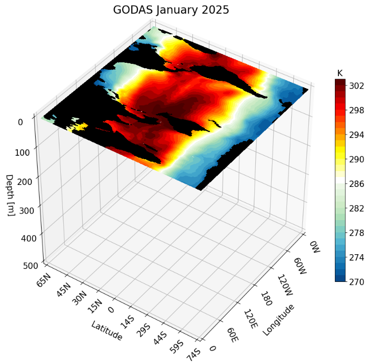
vmin, vmax = 270, 303 # min and max of colorbar
levels     = 34       # set how many colors you want to plot

# title for plot
title = f'GODAS January {year}'

# define depth index
depth_ind = 0 # depth to plot

We then call the function, making sure to close the figure afterward to free up memory:

fig = plot_depth_3D(title, temp, vmin, vmax, levels, depth_ind)
plt.show(fig)
plt.close(fig)

Surface

Global depth cross-sections at surface for January 2025.

Creating a GIF

We can call this function repeatedly, save each output as a PNG, and then combine the frames into a GIF. The setup is the same as above — the only difference is defining an array of depth indices to iterate over and adding a for loop:

#############################################################################
# -- Set up for function call -- #
# Set up global region
lat_cut_start = 0    
lat_cut_end = -1     
lon_cut_start = 0   
lon_cut_end = -1    
depth_cut_end = 28

# Defining the range and position of each tick for labeling
# last number changes the interval
lon_ticks   = np.arange(lon[lon_cut_start], lon[lon_cut_end]+2, 60) # adding 2 to get last tick
lat_ticks   = np.arange(lat[lat_cut_start], lat[lat_cut_end], 15)
lat_ticks[-1]   = np.ceil(lat[-1])   # add the last latitude point
depth_ticks = np.arange(0, depths[depth_cut_end], 100)

#############################################################################
# Set up for colorbar
vmin, vmax = 270, 303 # min and max of colorbar
levels     = 34       # set how many colors you want to plot

# title for plot
title = f'GODAS January {year}'

#############################################################################
# define indices
depths_to_plot = np.arange(depth_cut_end) # all depth layers to include in the animation

# -- Create PNGs -- #
######################################
pic_directory = os.getcwd()
# Call function and save PNG
for i, depth_ind in enumerate(depths_to_plot):
    fig    = plot_depth_3D(title, temp, vmin, vmax, levels, depth_ind)
    fn     = 'Depth_Cross_Section' + str(i) + '.png'
    fn     = os.path.join(pic_directory, fn)
    plt.savefig(fn, dpi=300, bbox_inches='tight')
    plt.close(fig)

# -- Create GIF -- #
######################################
gif_path = os.getcwd() # set GIF path
frame_files = []

# collect all saved cross-section figures
for i in range(len(depths_to_plot)):
  fn     = 'Depth_Cross_Section' + str(i) + '.png'
  fn     = os.path.join(pic_directory, fn)
  frame_files.append(fn)

output_path = os.path.join(gif_path, f'{title}_depth_animation.gif') # give GIF a name based on title

frames = [Image.open(frame).convert('RGB') for frame in frame_files] # load all frames
# save frames into one GIF
frames[0].save(
    output_path,
    save_all=True,
    append_images=frames[1:],
    duration=300,
    loop=0,
    optimize=False,  # Don't compress
    quality=500  # Maximum quality
)

# Delete the PNG files
for file in frame_files:
    os.remove(file)

print(f"{output_path} created!")

The resulting GIF steps through each depth layer from the surface down to approximately 500 meters, giving a clear picture of how ocean temperature varies with depth across the globe.

Depth anim

Global depth cross-sections for January 2025.

Zonal Cross-Section

The zonal cross-section is built in a similar way to the previous cross-section.

#############################################################################
#############################################################################
# Function will plot one zonal cross-section for a region
# Input
#         - title: string with tite for each figure
#         - data: 3D array with data to be visualized
#         - vmin, vmax: float clip value that defines maximum and minimum for the colorbar
#         - lat_ind: int with the latitude index that defines the cross-section
#         - levels: int that sets how many colors you want to plot
# Output
#         - fig: matplotlib figure object with the 3D figure
# Important variables
#         - lon_cut_start: int with starting longitude index
#         - lon_cut_end: int with end longitude index
#         - depth_cut_end: int with end depth index
# Note: make sure all tick values are defined before calling this function. This is
#       important for accurate labeling
#############################################################################
#############################################################################

def plot_zonal_3D(title, data, vmin, vmax, lat_ind, levels):

    # --- Setup Figure ---
    fig = plt.figure(figsize=(12, 13))
    fig.subplots_adjust(right = .95)  # Add this line
    
    title_sz = 20
    label_sz = title_sz-3
    
    ax = fig.add_subplot(111, projection='3d')       # This is what defines the plot as 3D
    
    # Contour Norms
    fixed_levels = np.linspace(vmin, vmax, levels)   # the colorbar ticks
    norm = mpl.colors.Normalize(vmin=vmin, vmax=vmax)
    
    # create grid for each lat, lon, and depth variable
    X, Y, Z = np.meshgrid(lon[lon_cut_start:lon_cut_end], lat[lat_cut_start:lat_cut_end], -depths[0:depth_cut_end])
    
    #############################################################################
    # plotting land for surface 
    surface3D = data[0, lat_cut_start:lat_cut_end,lon_cut_start:lon_cut_end]
    
    mask = np.isnan(surface3D) # create a mask for the NaN values
    masked_array = np.where(mask, surface3D, np.nan)          # change points with values to NaN
    masked_array = np.where(~mask, masked_array, vmin)        # change NaN points to values
    _ = ax.contourf(X[:, :, 0], Y[:, :, 0], masked_array, zdir='z', offset=-depths[0], cmap = mpl.colors.ListedColormap(['black']) ) # plotting the land
    # Contours
    #############################################################################
    # plotting the cross-section
    lat_depth3D = data[:depth_cut_end , lat_ind, lon_cut_start:lon_cut_end] # define the cross-section from the cut and index
    
    # plot the cross-section contour
    cs2 = ax.contourf(X[0, :, :], lat_depth3D.T, Z[0,:,:], zdir='y', levels=fixed_levels, cmap=newcmp2, offset= lat[lat_ind],
               norm = norm, extend = 'both')
    #############################################################################
    # plotting land for cross-section
    mask = np.isnan(lat_depth3D)                                # create a mask for the NaN values
    masked_array = np.where(mask, lat_depth3D, np.nan)          # change points with values to NaN
    masked_array = np.where(~mask, masked_array, vmin)          # change NaN points to values
    _ = ax.contourf(X[0, :, :], masked_array.T, Z[0,:,:], zdir='y', offset=lat[lat_ind], cmap = mpl.colors.ListedColormap(['black']) ) # plotting the land

    #############################################################################
    ax.grid(True)
    ax.set_xticks(lon_ticks, labels=[format_longitude(int(l)) for l in lon_ticks], fontsize=label_sz, rotation = -65, ha = 'left')  # Requires format_longitude function to remove degree symbol
    ax.set_yticks(lat_ticks, labels=[format_latitude(int(l)) for l in lat_ticks], fontsize=label_sz, rotation = 45, va = 'center')  # Requires format_latitude function to remove degree symbol
    ax.set_zticks(-depth_ticks, labels=[f"{t:.0f}" for t in depth_ticks], fontsize=label_sz)
    ax.tick_params(axis='x', pad=0, labelsize=label_sz)
    ax.tick_params(axis='y', pad=6,  labelsize=label_sz)
    ax.tick_params(axis='z', pad=7,  labelsize=label_sz)
    
    ax.set_xlabel('Longitude', fontsize=label_sz, labelpad=47)
    ax.set_ylabel('Latitude', fontsize=label_sz, labelpad=16)
    ax.set_zlabel('Depth [m]', fontsize=label_sz, labelpad=14, rotation=0)
    ax.set_title(title, fontsize=title_sz)
    
    # Set limits
    ax.set_xlim(lon_ticks[0], lon_ticks[-1])
    ax.set_ylim(lat_ticks[0], lat_ticks[-1])
    ax.set_zlim(-depth_ticks[-1], 0)
    
    #############################################################################
    ax.set_box_aspect((1, 1, 1))
    
    # view from above to make sure plot matches
    ax.view_init(elev=40, azim=-150, vertical_axis='z')
    #############################################################################
    #############################################################################
    # the colorbar for the data
    cbar = fig.colorbar(cs2, fraction=0.03, pad = 0, extendfrac=0)
    cbar.ax.set_title("K", fontsize = label_sz)
    cbar.ax.tick_params(labelsize=label_sz)    # set label size of ticks
    cbar.update_ticks()
    #############################################################################
    
    return fig

Let’s skip calling the function once and instead create the GIF. Unlike the high-resolution GLORYS data, GODAS has a coarse resolution. calling this function for a small region like the California coast looks pixelated.

Zonal Cali

Zonal cross-sections along California coast for January 2025.

Instead, we can use a larger region which does not require much detail and is perfect for this type of dataset. We use the North Pacific as an example:

# -- Set up for function call --
######################################
# Set up for the North Pacific
lat_cut_start = 134    # index for 30 S
lat_cut_end   = 405    # index for 60 N
lon_cut_start = 160    # index for 160 E
lon_cut_end   = 301    # index for 60 W
depth_cut_end = 27     # index for 459 meters

# Defining the range and position of each tick for labeling
# last number changes the interval
lon_ticks   = np.arange(lon[lon_cut_start], lon[lon_cut_end], 20)
lat_ticks   = np.round(np.arange(lat[lat_cut_start], lat[lat_cut_end], 10)) # round these because the scale is 1/3 and we want to round up
depth_ticks = np.arange(0, depths[depth_cut_end], 100) # if plotting the first 100 meters change the last number to something =<25

# Defining the latitudes to visualize
lat_indices = np.arange(lat_cut_start, lat_cut_end, 3)

# Set up for colorbar
vmin, vmax = 270, 303 # Change to scale better
colors     = 32       # set how many colors you want to plot

# title for plot
title = f'GODAS January {year}'

# -- Create PNG -- #
######################################
pic_directory = os.getcwd()
# create cross-section figures and save as PNG
for i, lat_ind in enumerate(lat_indices):
    fig = plot_zonal_3D(title, temp, vmin, vmax, lat_ind, colors)
    fn     = 'Zonal_Cross_Section' + str(i) + '.png'
    fn     = os.path.join(pic_directory, fn)
    plt.savefig(fn, dpi=300, bbox_inches='tight')
    plt.close(fig)

# -- Create GiF --
######################################
import imageio
from PIL import Image
import glob

gif_path = os.getcwd() # set GIF path
frame_files = []
# call all cross-section figures saved
for i in range(len(lat_indices)):
  fn     = 'Zonal_Cross_Section' + str(i) + '.png'
  fn     = os.path.join(pic_directory, fn)
  frame_files.append(fn)

output_path = os.path.join(gif_path, f'{title}_animation.gif') # give gif a name based on title

frames = [Image.open(frame).convert('RGB') for frame in frame_files] # put all figs together
# save figs
frames[0].save(
    output_path,
    save_all=True,
    append_images=frames[1:],
    duration=200,
    loop=0,
    optimize=False,  # Don't compress
    quality=500  # Maximum quality
)

# Delete the PNG files
for file in frame_files:
    os.remove(file)

print(f"{output_path} created!")

Zonal anim

Zonal cross-sections in Pacific region for January 2025. Written on March 24th, 2026 by Dani Lafarga