3D visualization of high-resolution climate data

Motivation

My previous 3D visualizations used Plotly, which was convenient and interactive, but it was limited in the amount of data it could handle. For my previous project, this was not an issue as the data was small.

3D OGCM

Multiple depths plotted for January climatology from OGCM.

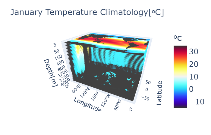
Once I started working with larger datasets, I found I was only able to plot one altitude layer of high-resolution data before crashing. This is when I turned to Python’s Matplotlib library and its 3D projection. It uses far less memory to create a figure and generates figures faster. Though I lost the interactive aspect (rotating, zooming in and out, etc.), I was still able to perform these tasks manually.

The following code is a tutorial for how to visualize 3D climate data using Matplotlib 3D projections. As an example, I use the first empirical orthogonal function (EOF) computed from the high-resolution Global Ocean Physics Reanalysis (GLORYS) output for all latitude-longitude-depth dimensions (3D) at once. The complete calculation for the GLORYS 3D EOFs can be found at this repository. The repository for the full code used in this tutorial is found at this GitHub repo.

Data and EOF Method

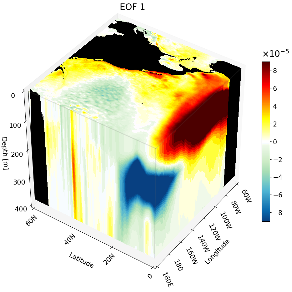
Here’s some of the nitty-gritty info for the example data used in this visualization. TLDR: we are plotting the first EOF (a spatial pattern) computed from large ocean temperature data (49 GB). You might recognize ENSO in the visualization — if you don’t know what that is, NOAA has a great breakdown. Look for a warm eastern tropical Pacific and cold western tropical Pacific.

The ocean temperature data in this study comes from the Global Ocean Physics Reanalysis (GLORYS), a high-resolution ($1/12^{\circ}$ by $1/12^{\circ}$) data assimilative global ocean simulation available from the Copernicus Marine Environment Monitoring Service. It has a spatial resolution of $1/12^{\circ}$ latitude by $1/12^{\circ}$ longitude with 50 depth layers covering the entire global ocean from $80^{\circ}$S to $90^{\circ}$N and $180^{\circ}$E to $180^{\circ}$W, extending from the ocean surface to 5,727 meters.

Table 1: The depth values of the 50 layers in the GLORYS model (unit: meters). Values were rounded to the first two decimal places.

0.49	1.54	2.65	3.82	5.08
6.44	7.93	9.57	11.41	13.47
15.81	18.50	21.60	25.21	29.44
34.43	40.34	47.37	55.76	65.81
77.85	92.33	109.73	130.67	155.85
186.13	222.51	266.04	318.13	380.21
453.94	541.09	643.57	763.33	902.34
1062.44	1245.29	1452.25	1684.28	1941.89
2225.08	2533.34	2865.70	3220.82	3597.03
3992.48	4405.22	4833.29	5274.78	5727.92

The EOFs are calculated across all dimensions (i.e., 3D EOFs) using a December-January-February (DJF) boreal winter mean of GLORYS ocean temperature data from 1993/1994 to 2020/2021, using the temporal covariance method. To manage computational memory costs, the matrix multiplication required for calculating temporal covariance and 3D EOFs is performed using a partitioned approach. For temporal covariance, partitioned segments of the transposed anomaly matrix are sequentially read in and multiplied by corresponding segments of the anomaly matrix until the full product is complete. Similarly, 3D EOFs are calculated by multiplying partitioned segments of the anomaly matrix with the eigenvectors of the temporal covariance matrix.

Visualization Setup

The visualization is broken up into 5 main sections:

Section 1: Depth cross-section — plots the data for a single depth layer
Section 2: Zonal cross-section — plots the data for a single latitude value
Section 3: Meridional cross-section — plots the data for a single longitude value
Section 4: All cross-sections plotted as a cube — combines all three cross-sections into one 3D figure
Section 5: Making a GIF — uses the zonal cross-section code in a function to create an animation of zonal cross-sections moving up the California coast

Here are the libraries you will need:

# all visualization libraries
import matplotlib as mpl
import matplotlib.pyplot as plt
from mpl_toolkits.mplot3d import Axes3D
from matplotlib import cm
from matplotlib.colors import ListedColormap, LinearSegmentedColormap

# to get path
import os

# libraries to read data
import netCDF4 as nc
from netCDF4 import Dataset as ds
import numpy as np

# libraries used for some math
from numpy import linspace
from numpy import meshgrid
import math

For the climate data I build a custom colormap:

# Creating the custom colormap
top2 = cm.get_cmap('GnBu_r')   # get green blue colormap
bottom2 = cm.get_cmap('hot_r') # get hot colormap
top_array = top2(np.linspace(0, 1, 128))        # create array with color values
bottom_array = bottom2(np.linspace(0, .9, 128)) # create array with color values
# edit array with color values to have better transition shades
top_array[-2:,:] = bottom_array[0,:]
top_array[-3,:] = np.array([1., 0.98823529, 1., 1.])
top_array[-4,:] = np.array([0.96862745, 0.98823529, 1., 1.])
top_array[-5,:] = np.array([0.96862745, 0.98823529, 0.94117647, 1.])

newcolors2 = np.vstack((top_array, bottom_array))         # stacking color arrays on top of each other
newcmp2 = ListedColormap(newcolors2, name='OrangeBlue')   # creating new colormap

To format the latitude and longitude axes I use two main functions that will add N (north) or S (south) to the latitudes and W (west) or E (east) to the corresponding longitudes.

#################################################################################################################
#################################################################################################################
# Function formats longitude to get rid of degree symbols
# Input:
#         - longitude: int with longitude from 0 to 360
# Output:
#         - string with longitude value and W (west) or E (east)
def format_longitude(longitude):
    if not 0 <= longitude <= 360:
        return "Invalid longitude. Must be between 0 and 360 degrees."

    if longitude == 0:
        hemisphere = ''
        degrees = longitude
    elif longitude < 180:
        hemisphere = 'E'
        degrees = longitude
    elif longitude == 180:
        hemisphere = ''
        degrees = longitude
    else:
        hemisphere = 'W'
        degrees = 360 - longitude

    return f"{degrees:.0f}{hemisphere}"

#################################################################################################################
#################################################################################################################

# Function formats latitude to get rid of degree symbols
# Input:
#         - latitude: int with latitude in degrees. Positive values are N and negative are S.
# Output:
#         - string with absolute value of latitude and S or N
def format_latitude(latitude):
    if not -90 <= latitude <= 90:
        return "Invalid latitude. Must be between -90 and 90 degrees."
# adding S or N based on negative or positive value
    if latitude > 0:
        hemisphere = "N"
    elif latitude == 0:
        hemisphere = ""
    else:
        hemisphere = 'S'

    degrees = abs(latitude)

    return f"{degrees:.0f}{hemisphere}"

There are three functions used to process the data:

get_var: Used to read in the latitude, longitude, and depth variables of the data we are plotting. This is heavily dependent on the variable names in the data file.
vol_weight: Used to calculate the volume at each grid point. This is important for correctly representing the data dimensions, but is not necessary for plotting. The EOF is weighted, meaning the volume is already multiplied in; this means we need to divide the volume out before visualization.
read_EOFs: Reads in the data file and divides out the volume weight at the end.

#################################################################################################################
#################################################################################################################
# Function get_var() will get variables that will be required for EOFs
# Input:
#         - fn: a string with the complete path of the data
# Output:
#         - lat: 1D array with all latitude values
#         - lon: 1D array with all longitude values
#         - depth: 1D array with all depth values
# NOTE: Change variable names according to your file
def get_var(fn):
    fn     =  ds(fn,'r')
    lat    = fn.variables['lat'][:].data    # read in latitude
    lon    = fn.variables['lon'][:].data    # read in longitude
    depths = fn.variables['depth'][:].data  # read in depth
    fn.close()
    return lat, lon, depths
#################################################################################################################
#################################################################################################################
# Function computes volume weights based on latitude and depth values. Although longitude values are not
# in the equation, the length of the longitude array is necessary for building the 3D volume weight array.
# Input:
#         - lat: 1D array with all latitude values
#         - lon: 1D array with all longitude values
#         - depth: 1D array with all depth values
# Output:
#         - area_weight: 3D array with volume weight
def vol_weight(depths, lon, lat):
    xx, yy = meshgrid(lon, lat)
    tot_depth = len(depths)
    # area weight for latitude values
    area_w = np.cos(yy*math.pi/180)
    if lat[-1] == 90.0:
        area_w[-1,:] = 0.0
    # volume weights for depth
    volume_weight = []
    for i in range(tot_depth):
        if i == 0:
            volume_weight.append(np.sqrt(depths[0] * area_w)) # first depth thickness
        else:
            volume_weight.append( np.sqrt((depths[i] - depths[i - 1]) * area_w))
    # Turning weights into one array
    volume_weight = np.array(volume_weight)
    return volume_weight
#################################################################################################################
#################################################################################################################
# Function will read one EOF mode
# Input:
#         - fn: string with the complete path of the data file
# Output:
#         - EOF: 3D float array with the EOF
def read_EOFs(fn):
  get_var(fn)
  EOF_ncfile = ds(fn, 'r')
  EOF = EOF_ncfile.variables['EOF']
  EOF = EOF[:].filled()
  EOF_ncfile.close()
  volume_weight = vol_weight(depths, lon, lat)
  EOF = EOF/volume_weight  # remember to divide by volume weight
  return EOF

To read in the EOFs, use os to navigate to the appropriate directory and then run:

# define the complete path with the file name
data_directory = os.getcwd()
fn     = 'EOF_1.nc'
fn     = os.path.join(data_directory, fn)

lat, lon, depths = get_var(fn) # read variables
EOF1 = read_EOFs(fn) # read EOF 1

Some Notes Before We Get Into Plotting Each Cross-Section

There is one main function that does most of the plotting. You can find the documentation for the function at https://matplotlib.org/stable/gallery/mplot3d/box3d.html.

For each of these plots, assume:

X-axis is longitude
Y-axis is latitude
Z-axis is depth

We define the variables X, Y, and Z as 3D arrays with their respective values, cropped to a specific region. To do this we use meshgrid with the order longitude, latitude, and depth. The meshgrid is built from the cropped dimensions to focus on a specific region.

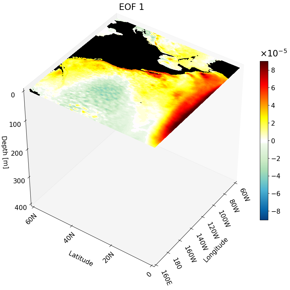
Visualizing One Depth Cross-Section

Here’s how we use the main function for the depth cross-section:

ax.contourf(X[:,:,0], Y[:,:,0], data, zdir='z', offset=-depths[0], levels=levels, cmap=newcmp2, norm=norm, vmin=vmin, vmax=vmax)

X and Y are 3D arrays with longitude, latitude, and depth values (in that order) cropped to a specified region. The indices below are defined to focus on the North Pacific:

lat_cut_start = 960    # index for the equator
lat_cut_end = 1681     # index for 60 N
lon_cut_start = 1920   # index for 160 E
lon_cut_end = 3601     # index for 60 W
depth_cut_end = 30     # index for 454 m

Since we are plotting on the Z axis, the depth value remains constant for every point, hence indexing with $[:,:,0]$. The value 0 is arbitrary here — X and Y are identical at every depth index.

data is a 2D (lat, lon) array derived from the EOF 3D array of shape (depth, lat, lon). Regardless of how it is indexed, depth will be held constant.

Note: The data array is always passed as the argument for the dimension that is held constant. Since depth is constant here, data is passed as the third argument.

The argument zdir specifies the direction in which the cross-section will be plotted. The offset should be a value along that same direction. In our example, since zdir = ‘z’ corresponds to depth, we set offset to the first depth value.

Note: The surface is defined as 0. Values above the surface are positive and values below are negative. Since our depth layers increase going deeper, we apply a negative sign to depth values when plotting.

The last four arguments control the colorbar, setting the colormap, normalization mapping, and the lower and upper limits, respectively.

Before plotting, we set up the region, crop the data, and define the dimension tick labels:

# Set up cube for the North Pacific
lat_cut_start = 960    # index for the equator
lat_cut_end = 1681     # index for 60 N
lon_cut_start = 1920   # index for 160 E
lon_cut_end = 3601     # index for 60 W
depth_cut_end = 30     # index for 454 m

# creating the depth cross-section surface
surface3D = EOF1[0, lat_cut_start:lat_cut_end, lon_cut_start:lon_cut_end]      # surface cross-section

# Defining the range and position of each tick for labeling
# last number changes the interval
lon_ticks   = np.arange(lon[lon_cut_start], lon[lon_cut_end], 20)
lat_ticks   = np.arange(lat[lat_cut_start], lat[lat_cut_end], 20)
depth_ticks = np.arange(0, depths[depth_cut_end], 100) # if plotting the first 100 meters change the last number to something =<25

# create grid for each lat, lon, and depth variable
X, Y, Z = np.meshgrid(lon[lon_cut_start:lon_cut_end], lat[lat_cut_start:lat_cut_end], -depths[0:depth_cut_end])

Now we plot the depth cross-section:

#############################################################################

# --- Setup Figure ---
fig = plt.figure(figsize=(11, 13))
title_sz = 20
label_sz = title_sz-5

ax = fig.add_subplot(111, projection='3d')  # This is what defines the plot as 3D
vmin, vmax = -0.00009, 0.00009              # Change to scale better
levels = 50                                 # set how many colors you want to plot

# Contour Norms
norm = mpl.colors.Normalize(vmin=vmin, vmax=vmax)
#############################################################################
# plot the surface depth cross-section
# offset will place the cross-section in the right position on the Z axis
cs2 = ax.contourf(X[:, :, 0], Y[:, :, 0], surface3D, zdir='z', offset=-depths[0],
                  levels=levels, cmap=newcmp2, norm=norm, vmin=vmin, vmax=vmax)
#############################################################################
# plotting land as black
mask = np.isnan(surface3D)                                                 # create a mask for the NaN values
masked_array = np.where(mask, surface3D, np.nan)                           # change points with values to NaN
end_of_map = np.nanmin(EOF1[31,lat_cut_start,lon_cut_start:lon_cut_end])   # minimum value to define bottom of map
masked_array = np.where(~mask, masked_array, end_of_map)                   # change NaN points to values
_ = ax.contourf(X[:, :, 0], Y[:, :, 0], masked_array, zdir='z', offset=-depths[0], cmap = mpl.colors.ListedColormap(['black']) ) # plotting the land as black

#############################################################################
# The following is VERY important
# It makes sure the bounds are defined accurately
# If your bounds are not defined well your plot will not show up!!!
# Formatting labels
ax.grid(False)
ax.set_xticks(lon_ticks, labels=[format_longitude(int(l)) for l in lon_ticks], fontsize=label_sz, rotation = -65, ha = 'left') # Requires format_longitude function to remove degree symbol
ax.set_yticks(lat_ticks, labels=[format_latitude(int(l)) for l in lat_ticks], fontsize=label_sz, rotation = 45)  # Requires format_latitude function to remove degree symbol
ax.set_zticks(-depth_ticks, labels=[f"{t:.0f}" for t in depth_ticks], fontsize=label_sz)
ax.tick_params(axis='x', pad=0, labelsize=label_sz)
ax.tick_params(axis='y', pad=0,  labelsize=label_sz)
ax.tick_params(axis='z', pad=7,  labelsize=label_sz)


# Label Axes
ax.set_xlabel('Longitude', fontsize=label_sz, labelpad=28)
ax.set_ylabel('Latitude', fontsize=label_sz, labelpad=16)
ax.set_zlabel('Depth [m]', fontsize=label_sz, labelpad=12, rotation=0)
ax.set_title("EOF 1", fontsize=title_sz)

# Set limits
ax.set_xlim(lon_ticks[0], lon_ticks[-1])
ax.set_ylim(lat_ticks[0], lat_ticks[-1])
ax.set_zlim(-depth_ticks[-1], 0)


#############################################################################

ax.set_box_aspect((1, 1, 1))
# view from above to make sure plot matches
ax.view_init(elev=40, azim=-145, vertical_axis='z')

#############################################################################
# the colorbar for the EOF data

sm = mpl.cm.ScalarMappable(norm=norm, cmap=newcmp2)
sm.set_array([])

cbar = fig.colorbar(sm, ax=ax, format = mpl.ticker.ScalarFormatter(useMathText=True), norm = norm, fraction=0.03, pad = 0)
cbar.ax.yaxis.get_offset_text().set_fontsize(title_sz) # change exp size
cbar.ax.yaxis.OFFSETTEXTPAD = 11           # moving exponent so it doesn't overlap with top of colorbar
cbar.ax.yaxis.set_offset_position('left')  # set exponent so it is more to the left
cbar.ax.tick_params(labelsize=label_sz)    # set label size of ticks
cbar.formatter.set_powerlimits((0, 0))     # formatting scientific notation
cbar.update_ticks()

depth

Depth cross-section at the surface for the North Pacific.

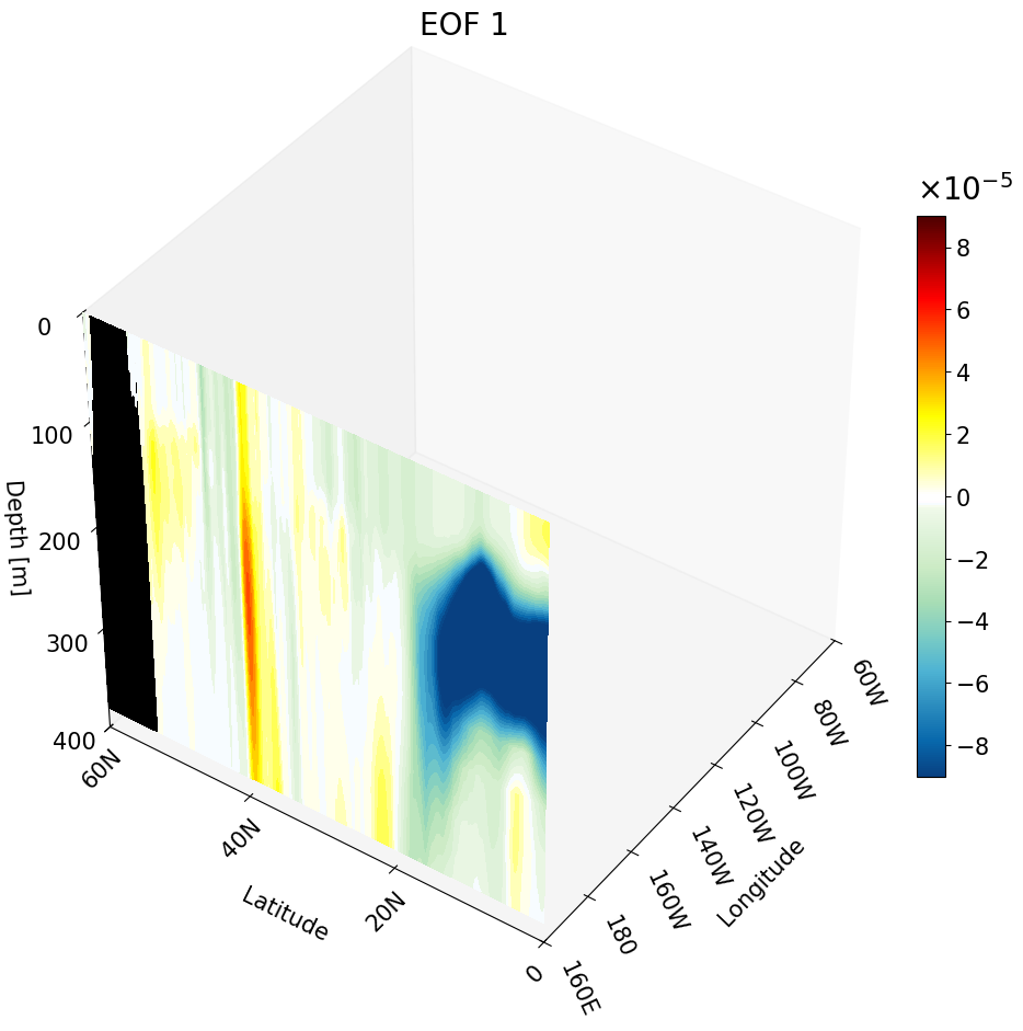
Visualizing One Zonal Cross-Section

We use the same main function with a few changes to produce a zonal cross-section:

ax.contourf(X[0, :, :], data, Z[0,:,:], zdir='y', offset=lat[lat_cut_start], levels=levels, cmap=newcmp2, norm=norm, vmin=vmin, vmax=vmax)

Now we hold latitude constant, which corresponds to the first index of X and Z. All values are the same throughout the first index, just as in the previous section. For consistency we plot at the first cut value using index 0.

zdir and offset are also updated to position the cross-section at the first latitude value for the North Pacific, lat[lat_cut_start], along the y-axis.

# Set up cube for the North Pacific
lat_cut_start = 960    # index for the equator
lat_cut_end = 1681     # index for 60 N
lon_cut_start = 1920   # index for 160 E
lon_cut_end = 3601     # index for 60 W
depth_cut_end = 30     # index for 454 m

# creating the zonal cross-section
lat_depth3D = EOF1[:depth_cut_end, lat_cut_start, lon_cut_start:lon_cut_end] # zonal cross-section

# Defining the range and position of each tick for labeling
# last number changes the interval
lon_ticks   = np.arange(lon[lon_cut_start], lon[lon_cut_end], 20)
lat_ticks   = np.arange(lat[lat_cut_start], lat[lat_cut_end], 20)
depth_ticks = np.arange(0, depths[depth_cut_end], 100) # if plotting the first 100 meters change the last number to something =<25

# create grid for each lat, lon, and depth variable
X, Y, Z = np.meshgrid(lon[lon_cut_start:lon_cut_end], lat[lat_cut_start:lat_cut_end], -depths[0:depth_cut_end])
#############################################################################
#############################################################################
#
#                      zonal cross-section figure
#
#############################################################################

# --- Setup Figure ---
fig = plt.figure(figsize=(11, 13))
title_sz = 20
label_sz = title_sz-5

ax = fig.add_subplot(111, projection='3d')  # This is what defines the plot as 3D
vmin, vmax = -0.00009, 0.00009              # Change to scale better
levels = 50                                 # set how many colors you want to plot

# Contour Norms
norm = mpl.colors.Normalize(vmin=vmin, vmax=vmax)
#############################################################################
# Plot zonal cross-section
ax.contourf(X[0, :, :], lat_depth3D.T, Z[0,:,:], zdir='y', levels=levels, cmap=newcmp2, offset= lat[960],
            norm=norm, vmin=vmin, vmax=vmax)

#############################################################################
# plotting land
mask = np.isnan(lat_depth3D)                                # create a mask for the NaN values
masked_array = np.where(mask, lat_depth3D, np.nan)          # change points with values to NaN
masked_array = np.where(~mask, masked_array, vmin)          # change NaN points to values
_ = ax.contourf(X[0, :, :], masked_array.T, Z[0,:,:], zdir='y', offset=lat[960], cmap = mpl.colors.ListedColormap(['black']) ) # plotting the land

#############################################################################
# The following is VERY important
# It makes sure the bounds are defined accurately
# If your bounds are not defined well your plot will not show up!!!
# Formatting labels
ax.grid(False)
ax.set_xticks(lon_ticks, labels=[format_longitude(int(l)) for l in lon_ticks], fontsize=label_sz, rotation = -65, ha = 'left') # Requires format_longitude function to remove degree symbol
ax.set_yticks(lat_ticks, labels=[format_latitude(int(l)) for l in lat_ticks], fontsize=label_sz, rotation = 45)  # Requires format_latitude function to remove degree symbol
ax.set_zticks(-depth_ticks, labels=[f"{t:.0f}" for t in depth_ticks], fontsize=label_sz)
ax.tick_params(axis='x', pad=0, labelsize=label_sz)
ax.tick_params(axis='y', pad=0,  labelsize=label_sz)
ax.tick_params(axis='z', pad=7,  labelsize=label_sz)


# Label Axes
ax.set_xlabel('Longitude', fontsize=label_sz, labelpad=28)
ax.set_ylabel('Latitude', fontsize=label_sz, labelpad=16)
ax.set_zlabel('Depth [m]', fontsize=label_sz, labelpad=12, rotation=0)
ax.set_title("EOF 1", fontsize=title_sz)

# Set limits
ax.set_xlim(lon_ticks[0], lon_ticks[-1])
ax.set_ylim(lat_ticks[0], lat_ticks[-1])
ax.set_zlim(-depth_ticks[-1], 0)


#############################################################################

ax.set_box_aspect((1, 1, 1))
# view from above to make sure plot matches
ax.view_init(elev=40, azim=-145, vertical_axis='z')

#############################################################################
# the colorbar for the EOF data

sm = mpl.cm.ScalarMappable(norm=norm, cmap=newcmp2)
sm.set_array([])

cbar = fig.colorbar(sm, ax=ax, format = mpl.ticker.ScalarFormatter(useMathText=True), norm = norm, fraction=0.03, pad = 0)
cbar.ax.yaxis.get_offset_text().set_fontsize(title_sz) # change exp size
cbar.ax.yaxis.OFFSETTEXTPAD = 11           # moving exponent so it doesn't overlap with top of colorbar
cbar.ax.yaxis.set_offset_position('left')  # set exponent so it is more to the left
cbar.ax.tick_params(labelsize=label_sz)    # set label size of ticks
cbar.formatter.set_powerlimits((0, 0))     # formatting scientific notation
cbar.update_ticks()

zonal

Zonal cross-section at the equator for the Pacific.

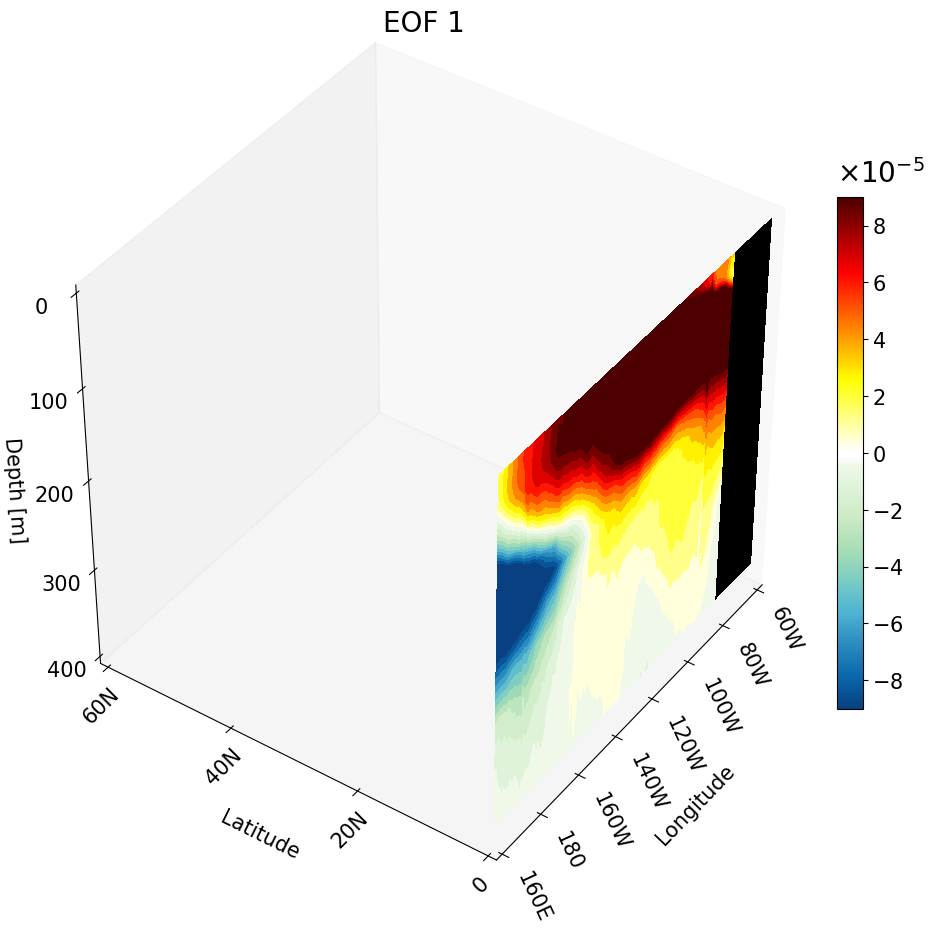
Visualizing One Meridional Cross-Section

We use the same main function with a few changes to produce a meridional cross-section:

ax.contourf(data, Y[:,0,:], Z[:,0,:], zdir='x', offset=lon_ticks[0], levels=levels, cmap=newcmp2, norm=norm, vmin=vmin, vmax=vmax)

Now we hold longitude constant, which corresponds to the second index of Y and Z.

zdir and offset are updated to position the cross-section along the x-axis at the first longitude tick value.

# Set up cube for the North Pacific
lat_cut_start = 960    # index for the equator
lat_cut_end = 1681     # index for 60 N
lon_cut_start = 1920   # index for 160 E
lon_cut_end = 3601     # index for 60 W
depth_cut_end = 30     # index for 454 m

# creating the meridional cross-section
lon_depth3D = EOF1[:depth_cut_end, lat_cut_start:lat_cut_end, lon_cut_start] # meridional cross-section

# Defining the range and position of each tick for labeling
# last number changes the interval
lon_ticks   = np.arange(lon[lon_cut_start], lon[lon_cut_end], 20)
lat_ticks   = np.arange(lat[lat_cut_start], lat[lat_cut_end], 20)
depth_ticks = np.arange(0, depths[depth_cut_end], 100) # if plotting the first 100 meters change the last number to something =<25

# create grid for each lat, lon, and depth variable
X, Y, Z = np.meshgrid(lon[lon_cut_start:lon_cut_end], lat[lat_cut_start:lat_cut_end], -depths[0:depth_cut_end])

#############################################################################
#############################################################################
#
#                      meridional cross-section figure
#
#############################################################################
#############################################################################

# --- Setup Figure ---
fig = plt.figure(figsize=(11, 13))
title_sz = 20
label_sz = title_sz-5

ax = fig.add_subplot(111, projection='3d')  # This is what defines the plot as 3D
vmin, vmax = -0.00009, 0.00009              # Change to scale better
levels = 50                                 # set how many colors you want to plot

# Contour Norms
norm = mpl.colors.Normalize(vmin=vmin, vmax=vmax)
#############################################################################
# plotting meridional cross-section
ax.contourf(lon_depth3D.T, Y[:, 0, :], Z[:, 0, :], zdir='x', offset=lon_ticks[0], levels=levels,
            cmap=newcmp2, norm=norm, vmin=vmin, vmax=vmax)
#############################################################################
# plotting land
mask = np.isnan(lon_depth3D) # create a mask for the NaN values
masked_array = np.where(mask, lon_depth3D, np.nan)          # change points with values to NaN
masked_array = np.where(~mask, masked_array, vmin) # change NaN points to values
_ = ax.contourf(masked_array.T, Y[:, 0, :], Z[:, 0, :], zdir='x', offset=lon_ticks[0], cmap = mpl.colors.ListedColormap(['black']) ) # plotting the land

#############################################################################
# The following is VERY important
# It makes sure the bounds are defined accurately
# If your bounds are not defined well your plot will not show up!!!
# Formatting labels
ax.grid(False)
ax.set_xticks(lon_ticks, labels=[format_longitude(int(l)) for l in lon_ticks], fontsize=label_sz, rotation = -65, ha = 'left') # Requires format_longitude function to remove degree symbol
ax.set_yticks(lat_ticks, labels=[format_latitude(int(l)) for l in lat_ticks], fontsize=label_sz, rotation = 45)  # Requires format_latitude function to remove degree symbol
ax.set_zticks(-depth_ticks, labels=[f"{t:.0f}" for t in depth_ticks], fontsize=label_sz)
ax.tick_params(axis='x', pad=0, labelsize=label_sz)
ax.tick_params(axis='y', pad=0,  labelsize=label_sz)
ax.tick_params(axis='z', pad=7,  labelsize=label_sz)


# Label Axes
ax.set_xlabel('Longitude', fontsize=label_sz, labelpad=28)
ax.set_ylabel('Latitude', fontsize=label_sz, labelpad=16)
ax.set_zlabel('Depth [m]', fontsize=label_sz, labelpad=12, rotation=0)
ax.set_title("EOF 1", fontsize=title_sz)

# Set limits
ax.set_xlim(lon_ticks[0], lon_ticks[-1])
ax.set_ylim(lat_ticks[0], lat_ticks[-1])
ax.set_zlim(-depth_ticks[-1], 0)


#############################################################################

ax.set_box_aspect((1, 1, 1))
# view from above to make sure plot matches
ax.view_init(elev=40, azim=-145, vertical_axis='z')

#############################################################################
# the colorbar for the EOF data

sm = mpl.cm.ScalarMappable(norm=norm, cmap=newcmp2)
sm.set_array([])

cbar = fig.colorbar(sm, ax=ax, format = mpl.ticker.ScalarFormatter(useMathText=True), norm = norm, fraction=0.03, pad = 0)
cbar.ax.yaxis.get_offset_text().set_fontsize(title_sz) # change exp size
cbar.ax.yaxis.OFFSETTEXTPAD = 11           # moving exponent so it doesn't overlap with top of colorbar
cbar.ax.yaxis.set_offset_position('left')  # set exponent so it is more to the left
cbar.ax.tick_params(labelsize=label_sz)    # set label size of ticks
cbar.formatter.set_powerlimits((0, 0))     # formatting scientific notation
cbar.update_ticks()

meridional

Meridional cross-section at 160E in the North Pacific.

All Cross-Sections Plotted as a Cube

Here we combine all three cross-sections into a single figure to form a cube. To do this, simply run each contourf command sequentially within the same figure. The code is annotated to clearly mark each section.

# Set up cube for the North Pacific
lat_cut_start = 960    # index for the equator
lat_cut_end = 1681     # index for 60 N
lon_cut_start = 1920   # index for 160 E
lon_cut_end = 3601     # index for 60 W
depth_cut_end = 30     # index for 454 m

# creating the cross-section arrays
surface3D   = EOF1[0, lat_cut_start:lat_cut_end, lon_cut_start:lon_cut_end]    # surface (depth) cross-section
lat_depth3D = EOF1[:depth_cut_end, lat_cut_start, lon_cut_start:lon_cut_end]   # zonal cross-section
lon_depth3D = EOF1[:depth_cut_end, lat_cut_start:lat_cut_end, lon_cut_start]   # meridional cross-section

# Defining the range and position of each tick for labeling
# last number changes the interval
lon_ticks   = np.arange(lon[lon_cut_start], lon[lon_cut_end], 20)
lat_ticks   = np.arange(lat[lat_cut_start], lat[lat_cut_end], 20)
depth_ticks = np.arange(0, depths[depth_cut_end], 100)

# create grid for each lat, lon, and depth variable
X, Y, Z = np.meshgrid(lon[lon_cut_start:lon_cut_end], lat[lat_cut_start:lat_cut_end], -depths[0:depth_cut_end])

# --- Setup Figure ---
fig = plt.figure(figsize=(11, 13))
title_sz = 20
label_sz = title_sz-5

ax = fig.add_subplot(111, projection='3d')
vmin, vmax = -0.00009, 0.00009 # Change to scale better
levels = 50

# Contours
norm = mpl.colors.Normalize(vmin=vmin, vmax=vmax)
#############################################################################
# plotting depth cross-section at the surface
cs2 = ax.contourf(X[:, :, 0], Y[:, :, 0], surface3D, zdir='z', offset=-depths[0],
                  levels=levels, cmap=newcmp2, norm=norm, vmin=vmin, vmax=vmax)
# plotting land
mask = np.isnan(surface3D) # create a mask for the NaN values
masked_array = np.where(mask, surface3D, np.nan)          # change points with values to NaN
end_of_map   = np.nanmin(EOF1[31,lat_cut_start,lon_cut_start:lon_cut_end]) # minimum value to define bottom of map
masked_array = np.where(~mask, masked_array, end_of_map)  # change NaN points to values
_ = ax.contourf(X[:, :, 0], Y[:, :, 0], masked_array, zdir='z', offset=-depths[0], cmap = mpl.colors.ListedColormap(['black']) ) # plotting the land

#############################################################################
# plotting zonal cross-section at the equator
ax.contourf(X[0, :, :], lat_depth3D.T, Z[0,:,:], zdir='y', levels=levels, cmap=newcmp2, offset=0,
            norm=norm, vmin=vmin, vmax=vmax)
# plotting land
mask = np.isnan(lat_depth3D) # create a mask for the NaN values
masked_array = np.where(mask, lat_depth3D, np.nan)      # change points with values to NaN
masked_array = np.where(~mask, masked_array, vmin)      # change NaN points to values
_ = ax.contourf(X[0, :, :], masked_array.T, Z[0,:,:], zdir='y', offset=0, cmap = mpl.colors.ListedColormap(['black']) ) # plotting the land

#############################################################################
# plotting meridional cross-section at 160E
ax.contourf(lon_depth3D.T, Y[:, 0, :], Z[:, 0, :], zdir='x', offset=lon_ticks[0], levels=levels,
            cmap=newcmp2, norm=norm, vmin=vmin, vmax=vmax)
# plotting land
mask = np.isnan(lon_depth3D) # create a mask for the NaN values
masked_array = np.where(mask, lon_depth3D, np.nan)          # change points with values to NaN
masked_array = np.where(~mask, masked_array, vmin) # change NaN points to values
_ = ax.contourf(masked_array.T, Y[:, 0, :], Z[:, 0, :], zdir='x', offset=lon_ticks[0], cmap = mpl.colors.ListedColormap(['black']) ) # plotting the land

#############################################################################
# formatting axes
ax.grid(False)
ax.set_xticks(lon_ticks, labels=[format_longitude(int(l)) for l in lon_ticks], fontsize=label_sz, rotation = -65, ha = 'left') # Requires format_longitude function to remove degree symbol
ax.set_yticks(lat_ticks, labels=[format_latitude(int(l)) for l in lat_ticks], fontsize=label_sz, rotation = 45)  # Requires format_latitude function to remove degree symbol
ax.set_zticks(-depth_ticks, labels=[f"{t:.0f}" for t in depth_ticks], fontsize=label_sz)
ax.tick_params(axis='x', pad=0, labelsize=label_sz)
ax.tick_params(axis='y', pad=0,  labelsize=label_sz)
ax.tick_params(axis='z', pad=7,  labelsize=label_sz)

ax.set_xlabel('Longitude', fontsize=label_sz, labelpad=28)
ax.set_ylabel('Latitude', fontsize=label_sz, labelpad=16)
ax.set_zlabel('Depth [m]', fontsize=label_sz, labelpad=12, rotation=0)
ax.set_title("EOF 1", fontsize=title_sz)

ax.set_xlim(lon_ticks[0], lon_ticks[-1])
ax.set_ylim(lat_ticks[0], lat_ticks[-1])
ax.set_zlim(-depth_ticks[-1], 0)

ax.set_box_aspect((1, 1, 1))
# view from above to make sure plot matches
ax.view_init(elev=40, azim=-145, vertical_axis='z')

#############################################################################
# soft edge lines to outline the cube
edges_kw = dict(color='0.4', linewidth=2, zorder=100, alpha=.16)

ax.plot(
    [lon[lon_cut_start], lon[lon_cut_end]],
    [lat[lat_cut_start], lat[lat_cut_start]],
    [-depths[0], -depths[0]],
    **edges_kw
)
ax.plot(
    [lon[lon_cut_start], lon[lon_cut_start]],
    [lat[lat_cut_start], lat[lat_cut_end]],
    [-depths[0], -depths[0]],
    **edges_kw
)
ax.plot(
    [lon[lon_cut_start], lon[lon_cut_start]],
    [lat[lat_cut_start], lat[lat_cut_start]],
    [-depths[0], -depths[depth_cut_end-1]],
    **edges_kw
)
# depth axis line to make depth extent obvious
ax.plot(
    [lon[lon_cut_start], lon[lon_cut_start]],
    [lat[lat_cut_end], lat[lat_cut_end]],
    [-depths[0], -depths[depth_cut_end-1]],
    **dict(color='0.1', linewidth=1, zorder=100)
)

#############################################################################
# the colorbar for the EOF data
sm = mpl.cm.ScalarMappable(norm=norm, cmap=newcmp2)
sm.set_array([])

cbar = fig.colorbar(sm, ax=ax, format = mpl.ticker.ScalarFormatter(useMathText=True), norm = norm, fraction=0.03, pad = 0)
cbar.ax.yaxis.get_offset_text().set_fontsize(title_sz) # change exp size
cbar.ax.yaxis.OFFSETTEXTPAD = 11           # moving exponent so it doesn't overlap with top of colorbar
cbar.ax.yaxis.set_offset_position('left')  # set exponent so it is more to the left
cbar.ax.tick_params(labelsize=label_sz)    # set label size of ticks
cbar.formatter.set_powerlimits((0, 0))     # formatting scientific notation
cbar.update_ticks()

cube

North Pacific with a depth, zonal, and meridional cross-section.

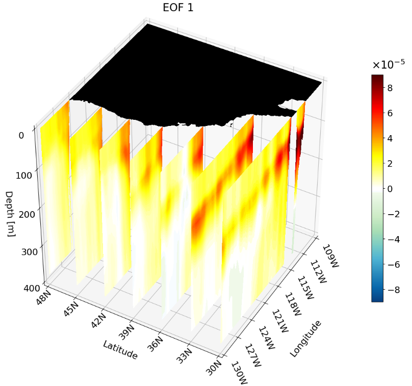
Multiple Cross-Sections Plotted at Once

As shown in the previous section, you can combine different cross-section types in a single figure. You can also plot multiple instances of the same cross-section type at once. This is particularly useful for publications, as it clearly shows how the climate signal changes with depth, latitude, or longitude.

For interpretability we take multiple zonal cross-sections along the California coast. This lets us see how ENSO drives warm anomalies along the coast and how the signal evolves moving northward.

The setup is the same as before, but we update the region indices to focus on 30°–48°N, 130°–109°W for approximately the first 400 meters:

lat_cut_start = 1320   # index for 30 N
lat_cut_end = 1537     # index for 48 N
lon_cut_start = 2760   # index for 130 W
lon_cut_end = 3013     # index for 109 W
depth_cut_end = 30     # index for 400 m

We also update the tick labels and meshgrid to match the new region:

# last number changes the interval
lon_ticks   = np.arange(lon[lon_cut_start], lon[lon_cut_end], 3)
lat_ticks   = np.arange(lat[lat_cut_start], lat[lat_cut_end], 3)
depth_ticks = np.arange(0, depths[depth_cut_end], 100) # if plotting the first 100 meters change the last number to something =<25

# create grid for each lat, lon, and depth variable
X, Y, Z = np.meshgrid(lon[lon_cut_start:lon_cut_end], lat[lat_cut_start:lat_cut_end], -depths[0:depth_cut_end])

Most importantly, we define the latitude indices for the zonal cuts we wish to visualize. Here I create a simple array containing an index for every third degree from 30°–48°N:

lat_indices = np.arange(lat_cut_start, lat_cut_end, 12*3)

The rest of the figure creation is essentially the same as the single zonal cross-section, with one key difference: we iterate through the latitude index array to plot a contour at each latitude slice.

# plotting the multiple cross-sections
for i, lat_ind in enumerate(lat_indices):
    lat_depth3D = EOF1[:depth_cut_end, lat_ind, lon_cut_start:lon_cut_end] # define the cross-section from the cut and index
    
    # plot the cross-section contour
    C = ax.contourf(X[0, :, :], lat_depth3D.T, Z[0,:,:], zdir='y', levels=levels, cmap=newcmp2, offset=lat[lat_ind],
              norm=norm, vmin=vmin, vmax=vmax)

The complete figure code is:

# --- Setup Figure ---
fig = plt.figure(figsize=(11, 13))
fig.subplots_adjust(right=.95)

title_sz = 20
label_sz = title_sz-3

ax = fig.add_subplot(111, projection='3d')  # This is what defines the plot as 3D

clip = 0.00009                              # clip value
title = 'EOF 1'

vmin, vmax = -clip, clip                    # Change to scale better
levels = 50                                 # set how many colors you want to plot

# Contour Norms
norm = mpl.colors.Normalize(vmin=vmin, vmax=vmax)

#############################################################################
# plotting land at the surface
surface3D = EOF1[0, lat_cut_start:lat_cut_end, lon_cut_start:lon_cut_end]

mask = np.isnan(surface3D) # create a mask for the NaN values
masked_array = np.where(mask, surface3D, np.nan)          # change points with values to NaN
masked_array = np.where(~mask, masked_array, vmin) # change NaN points to values
_ = ax.contourf(X[:, :, 0], Y[:, :, 0], masked_array, zdir='z', offset=-depths[0], cmap = mpl.colors.ListedColormap(['black']) ) # plotting the land

#############################################################################
# plotting the multiple cross-sections
for i, lat_ind in enumerate(lat_indices):
    lat_depth3D = EOF1[:depth_cut_end, lat_ind, lon_cut_start:lon_cut_end] # define the cross-section from the cut and index
    
    # plot the cross-section contour
    C = ax.contourf(X[0, :, :], lat_depth3D.T, Z[0,:,:], zdir='y', levels=levels, cmap=newcmp2, offset=lat[lat_ind],
              norm=norm, vmin=vmin, vmax=vmax)
#############################################################################
ax.grid(True)
ax.set_xticks(lon_ticks, labels=[format_longitude(int(l)) for l in lon_ticks], fontsize=label_sz, rotation = -65, ha = 'left')  # Requires format_longitude function to remove degree symbol
ax.set_yticks(lat_ticks, labels=[format_latitude(int(l)) for l in lat_ticks], fontsize=label_sz, rotation = 45, va = 'center')  # Requires format_latitude function to remove degree symbol
ax.set_zticks(-depth_ticks, labels=[f"{t:.0f}" for t in depth_ticks], fontsize=label_sz)
ax.tick_params(axis='x', pad=0, labelsize=label_sz)
ax.tick_params(axis='y', pad=6,  labelsize=label_sz)
ax.tick_params(axis='z', pad=7,  labelsize=label_sz)

ax.set_xlabel('Longitude', fontsize=label_sz, labelpad=47)
ax.set_ylabel('Latitude', fontsize=label_sz, labelpad=16)
ax.set_zlabel('Depth [m]', fontsize=label_sz, labelpad=14, rotation=0)
ax.set_title(title, fontsize=title_sz)

# Set limits
ax.set_xlim(lon_ticks[0], lon_ticks[-1])
ax.set_ylim(lat_ticks[0], lat_ticks[-1])
ax.set_zlim(-depth_ticks[-1], 0)

#############################################################################
ax.set_box_aspect((1, 1, 1))

# view from above to make sure plot matches
ax.view_init(elev=40, azim=-150, vertical_axis='z')
#############################################################################
# the colorbar for the EOF data
sm = mpl.cm.ScalarMappable(norm=norm, cmap=newcmp2)
sm.set_array([])

cbar = fig.colorbar(sm, ax=ax, format = mpl.ticker.ScalarFormatter(useMathText=True), norm = norm, fraction=0.03, pad=.05)
cbar.ax.yaxis.get_offset_text().set_fontsize(title_sz) # change exp size
cbar.ax.yaxis.OFFSETTEXTPAD = 11           # moving exponent so it doesn't overlap with top of colorbar
cbar.ax.yaxis.set_offset_position('left')  # set exponent so it is more to the left
cbar.ax.tick_params(labelsize=label_sz)    # set label size of ticks
cbar.formatter.set_powerlimits((0, 0))     # formatting scientific notation
cbar.update_ticks()

multi zonal

Multiple zonal cross-sections for the California coast. Written on February 2nd , 2026 by Dani Lafarga