import numpy as np
from numpy import meshgrid
import scipy.io as sc
import os
from pprint import pprint
import matplotlib.pyplot as plt
import scipy.linalg as la
import pandas as pd
from numpy import linspace
from numpy import meshgrid
from mpl_toolkits.basemap import Basemap
import matplotlib

from matplotlib import cm
from matplotlib.colors import ListedColormap, LinearSegmentedColormap
# this is for formatting the colorbar for every plot
bottom2 = cm.get_cmap('winter', 128)   # get winter colorbar to use for bottom half of colorbar
top2 = cm.get_cmap('hot_r', 128)       # get revers hot colorbar to use for top half of colorbar

newcolors2 = np.vstack((bottom2(np.linspace(0, 1, 128)),
                    top2(np.linspace(0, .9, 128))))       # stack colorbars on top of each other
newcmp2 = ListedColormap(newcolors2, name='OrangeBlue')   # name new colorbar newcmp2

### Defining Constants 

depths = [5, 10, 20, 30, 50, 75, 100, 125, 150, 200, 250, 300, 400, 500, 600, 700, 800, 900, 1000, 1100, 1200, 1300, 1400, 1500, 1750, 2000, 3000, 3500, 4000, 4500, 5000, 5500]
tot_depths = len(depths)
month = 'Jan'

## Reading in all the data

This model data from JPL’s non-Boussinesq ocean general circulation model (OGCM).
This data is downloaded from github and is only for the month of January

url = 'https://media.githubusercontent.com/media/dlafarga/calc_3D_EOFs/main/OGCM/Jan_ogcm.csv' # URL with Jan OGCM
data_T = pd.read_csv(url,header = None) # read in url
data_T = np.mat(data_T) # turn file into a Matrix
data_T = data_T.squeeze() # remove unnecessary 1 dimension 

data_T.shape

## Compute Standard Deviation and Climatology

N = data_T.shape[0] # total number of points
Y = data_T.shape[1] # total number of years

np.nanmean and np.nanstd computes the average and standard deviation for the rows (hence axis = 1) of the data. The command takes into account the NaNs for the data

import warnings

# I expect to see RuntimeWarnings in this block

with warnings.catch_warnings():
    warnings.simplefilter("ignore", category=RuntimeWarning)
    clim = np.nanmean(data_T, axis = 1)   # climatology  
    sdev = np.nanstd(data_T, axis = 1)    # standard deviation
clim_sdev = np.column_stack((clim, sdev)) # save this as one matrix 

## Compute anomalies

Details of computing anomalies is in this post https://dlafarga.github.io/journal/python_start.html


anom = data_T - clim
anom.shape

### Calc Standardized Anom

Standardized anomalies are anomalies divided by standard deviation
These are not used in the computation because it will amplify errors due to the nature of the data
Section was only added for completeness. 

np.seterr(divide='ignore', invalid='ignore') # runtime error will appear because of truncation
stnd_anom = anom/sdev

## Compute area weighted Anom

Each Anom has to be multiplied by a weight to project data onto a physical surface. This weight takes into account lattitude and thickness of depth. 

import math

# lattitude values
x = linspace(0, 360-1, 360)
y = linspace(-90, 90-1, 180)

xx, yy = meshgrid(x, y)
y_temp = yy.flatten()

# area weight for lattitude values
area_w = np.cos(y_temp*math.pi/180)

# area weights for depth
area_weight = []

for i in range(tot_depths):
    if i == 0:
        area_weight.append(np.sqrt(5 * area_w)) # first depth thickness is just 0-5m
    else:
        area_weight.append( np.sqrt((depths[i] - depths[i - 1]) * area_w))

# Turning weights into one array
area_weight = np.mat(area_weight)
area_weight = area_weight.flatten()
area_weight = area_weight.T
area_weight.shape

# Multiply area weight
weighted_A = np.empty((N,Y)) * np.nan # new array of weighted anomalies
weighted_A = np.multiply(anom , area_weight) # multiply weights and anomalies
weighted_A.shape

##  Compute EOFs Using SVD

This will compute EOFs using SVD. This is for small data sets and only to verify the method proposed. 

from eofs.standard import Eof

dat = np.array(weighted_A.T) # solver only takes in arrays

solver = Eof(dat) # define solver

# Find eigenvalues
# These eigenvalues are scaled by Y
eigenvalues = solver.eigenvalues()
eigenvalues = eigenvalues * Y # multiply by Y to get same Eigenvalues as temporal covariance 

eofs = solver.eofs() # compute EOFs 
eofs = eofs.T
eofs.shape

eofs = eofs/area_weight[:,0] # get physical EOFs (without weight)

#Plot EOF
plt.figure(figsize=(15., 7.))

title_sz = 25
label_sz = 20
exp_sz = 18

mymap = Basemap(projection='cyl', lon_0 = 180, lat_0 = 0) 

x = linspace(0, 360, 360)
y = linspace(-90, 90, 180)

xx, yy = meshgrid(x, y)


mode = 0  # CHANGE MODE HERE
depth_ind  = 9 # CHANGE DEPTH HERE
depth = depths[depth_ind]


EOF1 = np.reshape(eofs[depth_ind *64800: (depth_ind+1) *64800, mode],(180,360))
clip = .0004 # set min and max values
EOF1 = np.maximum(np.minimum(EOF1, clip), -clip) # climp min and max values


mymap.drawcoastlines(color='black', linewidth=.5)
mymap.drawmapboundary()

plt.contourf(xx, yy, -EOF1, 25 ,cmap = newcmp2)
plt.title('EOF mode '+ str(mode+1) + ' for '+month+' with depth of ' + str(depth) + 'm', fontsize=title_sz)

mymap.drawparallels(np.arange(-90,90,30), labels = [1,0,0,0],fontsize = label_sz) # draw lines and labels for latitudes
mymap.drawmeridians(np.arange(-180,180,60), labels = [0,0,0,1],fontsize= label_sz)# draw lines and labels for lomgitudes

cbar = plt.colorbar(shrink = .95, format = matplotlib.ticker.ScalarFormatter(useMathText=True)) # make colorbar fit size of graph
cbar.ax.yaxis.get_offset_text().set_fontsize(exp_sz) # change exp size
cbar.ax.yaxis.OFFSETTEXTPAD = 11           # moving exponent so it doesnt overlap with top of colorbar
cbar.ax.yaxis.set_offset_position('left')  # setexponent so it is more left 
cbar.ax.tick_params(labelsize=label_sz)    # set label size of ticks
cbar.formatter.set_powerlimits((0, 0))     # formatting scientific notation
cbar.update_ticks()

plt.show()

pcs = solver.pcs() # Solve for PCs

# Normalize
for col_i in range(54):
    pcs[:,col_i] = pcs[:,col_i] / np.linalg.norm(pcs[:,col_i])

## Getting rid of NaN in anom

NaN needs to be removed from the data to compute covariance, eigenvalues, and eigenvectors

# find which indicies have data (are not NaN)
numrows = np.argwhere(np.isnan(weighted_A[:,0]) == False)
new_N = round(numrows.shape[0]) # new N dimension without NaNs

# Create matrix with only values
new_anom = np.empty((new_N,Y)) * np.nan
for i in range(new_N):
        new_anom[i,:] = weighted_A[numrows[i,0],:]
new_anom = np.mat(new_anom)
new_anom.shape

# how much of the data is data?
new_N/N

## Compute Covariance

see https://dlafarga.github.io/journal/python_start.html for specifics on calculation

cov = (new_anom.T * new_anom)
# should have Y by Y matrix
cov.shape

## Computing Eigenvalues and Eigenvectors

see https://dlafarga.github.io/journal/python_start.html for specifics on calculation

important notes for np.linalg.eig:
    
    in  eigvals, eigvecs = np.linalg.eig(cov)
    The eigenvalues are not necessarily ordered
    the column eigves[:,i] is the eigenvector corresponding to the eigenvalue eigvals[i].

eigvals, eigvecs = np.linalg.eig(cov)

eigvecs = np.array(eigvecs)
eigvecs.shape

# Check to make sure vectors are orthogonal
# this will raise error if they aren't
n, m = eigvecs.shape
for col_i in range(m):
    for col_j in range(m):
        if col_i < col_j:  # use strictly less than because we don't want to consider a column with itself, and the dot product is commutable so order doesn't matter
            is_orthogonal = np.dot(eigvecs[:, col_i], eigvecs[:, col_j])
            if not np.isclose(is_orthogonal, 0):
                raise ValueError(f"Eigenvector {col_i} and Eigenvector {col_j} are not orthogonal.")

# checking magnitude of EOF. If magnitude is not one error will be raised
for col_i in range(54):
    is_one = np.linalg.norm(eigvecs[:,col_i])
    if not np.isclose(is_one, 1):
        raise ValueError(f"EOF {col_i} is not one")

eigvecs = np.mat(eigvecs)

Sorting Eigenvalues and Eigenvectors

eig_index = np.argsort(eigvals) # indexes with correct sorted order
eig_index = np.flip(eig_index)

new_eigvals = eigvals[eig_index[:]] # reorder evals
eigvals = new_eigvals

new_eigvecs = eigvecs[:,eig_index] # reorder evecs
eigvecs = new_eigvecs 

### Principle Component Plot

plt.figure(figsize=(13., 7.))
mode = 1

title_sz = 25
label_sz = 20
tick_sz = 5
line = 3

time = np.arange(1950,2004)

if eigvecs[0,mode-1] is not pcs[0,mode-1]:
    eigvecs[:,mode-1] = 0 - eigvecs[:,mode-1]

plt.plot(time, eigvecs[:,mode-1],'b', marker = 'o',label = 'PC with Cov',linewidth=line, markersize = line+5)
plt.title(month + ' PC ' + str(mode) , fontsize = title_sz)

plt.xticks(fontsize = label_sz)
plt.yticks(fontsize = label_sz)
plt.xlabel('Year', fontsize = label_sz)

plt.show()

### Scree Plot

num_eval = np.arange(eigvals.shape[0])+1 # mode numbers

cumulative_eval = np.cumsum(eigvals) # compute cummulative variance

fig, ax = plt.subplots()

fig.set_size_inches(11., 7.)
title_sz = 25
label_sz = 20
tick_sz = 5
# plotting Percentage Variance
p1, = plt.plot(num_eval,(eigvals/cumulative_eval[-1])*100, 'b',marker = 'o',label = 'Percentage Variance')
# formatting for left axis
ax.set_ylabel("Percentage Variance", size = label_sz)
ax.tick_params('y', colors='b',size = tick_sz, labelsize = label_sz-2)
ax.yaxis.label.set_color('blue')
plt.xticks(fontsize= label_sz-2)

# plotting Cummulative Percentage Variance
ax2 = ax.twinx()
p2, = plt.plot(num_eval,(cumulative_eval/cumulative_eval[-1])*100,'r',marker = 'x',label = 'Cumulative Percentage Variance')

# formatting for right axis
ax2.tick_params('y', colors='r',size = tick_sz, labelsize = label_sz-2)
ax2.set_ylabel("Cumulative Percentage Variance", size = label_sz)
ax2.yaxis.label.set_color('red')


plt.legend(handles=[p1,p2],loc='center right', fontsize = label_sz-5)
plt.title(month+ ' Scree Plot', size = title_sz)

plt.show()

## Computing EOF

see https://dlafarga.github.io/journal/python_start.html for specifics on calculation

### A*v

ev = eigvecs.T

EOFs = []
for j in range(Y):
    EOFs.append(np.matmul(weighted_A , ev[j].T))

EOF = np.array(EOFs)
EOF = np.squeeze(EOF)

EOF = EOF.T
EOF.shape

### Getting rid of NaN

This is done to find magnitude of EOFs

na_rows = np.argwhere(np.isnan(EOF[:,0]) == False) # find which rows have numbers
new_N = round(na_rows.shape[0]) # define new spatial dimension

# fill new matrix with no NaNs
new_EOF = np.empty((numrows.shape[0],Y))*np.nan
for i in range(numrows.shape[0]):
        new_EOF[i,:] = EOF[numrows[i,0],:]
new_EOF = np.mat(new_EOF)
new_EOF.shape

### Find Magnitude and divide

mag = np.linalg.norm(new_EOF, axis = 0)

for i in range(Y):
    EOF[:,i] = EOF[:,i]/mag[i]

### Varifying Geometric EOFs

new_EOF = np.empty((numrows.shape[0],Y))*np.nan 
for i in range(numrows.shape[0]):
        new_EOF[i,:] = EOF[numrows[i,0],:]
new_EOF.shape

# Check to make sure vectors are orthogonal
n, m = new_EOF.shape
for col_i in range(m):
    for col_j in range(m):
        if col_i < col_j:  # use strictly less than because we don't want to consider a column with itself, and the dot product is commutable so order doesn't matter
            is_orthogonal = np.dot(new_EOF[:, col_i], new_EOF[:, col_j])
            if not np.isclose(is_orthogonal, 0) and col_j != 53:
                pprint(f"EOF Mode {col_i} and EOF Mode {col_j} are not orthogonal.")
                pprint(np.dot(new_EOF[:, col_i], new_EOF[:, col_j]))
                

# checking magnitude of EOF. If magnitude is not one error will be raised
for col_i in range(Y):
    is_one = np.linalg.norm(new_EOF[:,col_i])
    if not np.isclose(is_one, 1):
        raise ValueError(f"EOF {col_i} is not one")

### Compute Physical EOFs

Now that  we have computed geometric EOFs we need to compute Physical EOFs by dividing by the volume weights. 

EOF = EOF/area_weight[:,0]

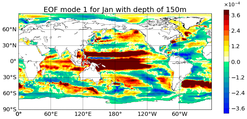
### Plot  Physical EOF

#Plot EOF
plt.figure(figsize=(15., 7.))

mymap = Basemap(projection='cyl', lon_0 = 180, lat_0 = 0) 

x = linspace(0, 360, 360)
y = linspace(-90, 90, 180)

xx, yy = meshgrid(x, y)


mode = 0
depth_ind  = 8
depth = depths[depth_ind]


EOF1 = np.reshape(EOF[depth_ind *64800: (depth_ind+1) *64800, mode],(180,360))
clip = .0004 # set min and max values
EOF1 = np.maximum(np.minimum(EOF1, clip), -clip) # climp min and max values

mymap.drawcoastlines(color='black', linewidth=.5)
mymap.drawmapboundary()

plt.contourf(xx, yy, -EOF1, 25 ,cmap = newcmp2)
plt.title('EOF mode '+ str(mode+1) + ' for '+month+' with depth of ' + str(depth) + 'm', fontsize=title_sz)

mymap.drawparallels(np.arange(-90,90,30), labels = [1,0,0,0],fontsize = label_sz) # draw lines and labels for latitudes
mymap.drawmeridians(np.arange(-180,180,60), labels = [0,0,0,1],fontsize= label_sz)# draw lines and labels for lomgitudes

cbar = plt.colorbar(shrink = .95, format = matplotlib.ticker.ScalarFormatter(useMathText=True)) # make colorbar fit size of graph
cbar.ax.yaxis.get_offset_text().set_fontsize(exp_sz) # change exp size
cbar.ax.yaxis.OFFSETTEXTPAD = 11           # moving exponent so it doesnt overlap with top of colorbar
cbar.ax.yaxis.set_offset_position('left')  # setexponent so it is more left 
cbar.ax.tick_params(labelsize=label_sz)    # set label size of ticks
cbar.formatter.set_powerlimits((0, 0))     # formatting scientific notation
cbar.update_ticks()

plt.show()