Computing 3D EOFs Using Covariance in Time and Singular Value Decomposition in Python

Motivation

Existing oceanic studies on either data reconstruction or dynamics often used 2-dimensional empirical orthogonal functions (EOF) for sea surface temperature (SST) and for deep layers. However, large-scale oceanic dynamics, such as equatorial ocean upwelling and arctic ocean ventilation, implies the existence of strong covariance among the temperatures and other parameters of different layers. These ocean dynamics are not best represented in the isolated 2-dimensional calculations layer-by-layer, while the 3-dimensional EOFs have a clear advantage.

For the purpose of this example we will be using NASA JPL ocean general circulation model (OGCM) on a 1 by 1 degree grid to accomplish our goal of quatifying significant deeper ocean dynamics by performing a 3D calculation. Although the SVD method could be applied here it is not ideal for data with higher resolution. We propose a method that will be applicable to most datasets as a way of making such a goal accessible and accommodating. Nevertheless SVD is a powerfull tool and will be used in tandem with temporal covariance to verify these results. To download the full code to compute 3D EOFs see this github repository.

Background

What is covariance?

Covariance measures how much two variables change. Typically in climatology covariance is considered between stations, grid boxes, or grid points. Covariance between two grid boxes i and j can be denoted as:

For N grid boxes covariance would be an N by N matrix:

Consider data a data matrix X that consists of N stations and Y time steps:

Climatology is computed as:

Our anomalies are computed as follows: \(A_{N \times Y} = [a_{it}]_{N\times Y} = [x_{it} - \bar x_{i}]_{N\times Y}\)

These anomalies are multiplied by their spatial weights to better reflect the geometric sizes of their corresponding grid boxes. A 3D grid box in the equator region is much larger than one in the polar region. In 2D the weight is related to the area of a grid box. Naturally, in our 3D case the weightfor a 3D grid box $i$ should be related to the volume of the grid box:

where \(\Delta d_i\) is the thickness of the layer for the grid box \(i\) and \(\phi_i\) [radians] is the latitude of the grid box \(i\). The square root is needed due to the symmetry of the formulation of the eigenvalue problem of a covariance matrix (Shen (2017)). Note: For purposes of this proof we assume that our spatially weighted anomaly matrix has no NaNs and is only filled with actual data. If there are NaNs you will need to remove them after this step!

Covariance in space is defined as:

Similarly covariance in time, temporal covariance can be defined as:

The difference between spatial covariance and temporal covariance is instead of computing the covariance between each grid box we are computing the covariance between the same grid box for different years given a specific month. We can use either of the two to find EOFs with the latter being the more efficient of the two.

What are Empirical Orthogonal functions?

Emperical orthogonal functions are eigenvectors. Eigenvectors are vectors that point in the same direction as their corresponding matrix.

Consider the square covariance matrix \([\sum_{ij}]_{N\times N}\) and some vector \(\vec{u}\) which runs parallel to \([\sum_{ij}]_{N\times N}\). There is a scalar or eigenvalue \(\rho\) which scales \(\vec{u}\) such that:

The first few eigenvectors of a climate covariance matrix from climate data often represent some typical patterns of climate variability (Shen and Somerville(2019)). In short EOFs will not only show climate patterns, but will quantifiably explain their importance.

Proof of Covariance in Time and EOFs

Consider some data \(x_{it}\) whose anomalies are \(A_{N\times Y}\) their spatial covariance is then:

and their covarience with respect to time is:

In space there is some vector \(\vec{v}\) that points in the same direction as \([C_{ij}]_{N\times N}\) such that

In time there is some other vector \(\vec{v}\) that points in the same direction as \([\sum _{tt'}]_{Y\times Y}\) such that:

Meaning \(\vec{u}\) are the eigenvectors of \([\sum _{ij}]_{N\times N}\) with \(\rho\) being it’s eigenvalues, and \(\vec{v}\) are the eigenvectors of \([\sum _{tt'}]_{Y\times Y}\) with \(\lambda\) being it’s eigenvalues.

The problem we are trying to answer is how these eigenvectors and eigenvalues relate? Above we defined covariance in time as \([\sum_{tt'}]_{Y\times Y} = \frac1 N A_{Y\times N}^T A_{N\times Y}\). We can ignore the 1/N as this will only scale the unique vector and not change its direction. Therefore:

plugging this into its eigenvalue problem:

Multiply both sides by A:

because \([\sum _{ij}]_{N\times N} = A_{N\times Y} A_{Y\times N}^T\) we can redefine the equation above as:

let \(\vec{w} = A_{N\times Y} \vec{v}\) this gives:

This is similar to: \([\sum _{ij}]_{N\times N} \vec{u} = \rho \vec{u}\)

Comparing the two equations we can conclude: \(\rho = \lambda\) and \(\vec{w} = A \vec{v}\). \(\vec{w}\) does not equal to one so it needs to be normalized. To do this we divide it by its magnitude

Quick SVD note

I will be using the EOF Solver(Dawson (2016)) to compute SVD. If you would like the full derivation of the documentation see here. You can also see the specifics of the function here.

The OGCM Data

Each case will be different so as an example I will take one month (January) of OGCM data to explain what this program is expecting of the data matrix. There are a few things that need to be considered for our OGCM data: - One month of data is taken from 1950 to 2003 therefore there is a total of 54 years or Y = 54. - Each month has latitude x longitude x depth - Latitude and Longitude are on 1 x 1 degree grid - Latitude spans 89.5 S to 89.5 N - Longitude is centered at 180 can be said to do from 0 to 360 - depths are from 5m to 5,500m and split up into 32 depths - The total amount of grid points are \(N = 180(latitude) \times 360 (Longitude) \times 32 = 2,073,600\)

Initially one month of data is a multidimensional matrix, if we were to take one year and one layer of the month of January it looks like:

This is flattened and later transposed to a column array. The flattened row version looks like:

Again this is then transposed to be the column array $\vec{T}{l_1, Y{1950}}$. Each layer is put into the same row and each column is the same year. The resulting data matrix that we call data_T is then:

Remember each \(\vec{T}_{l_1, Y_{1950}}\) is an array containing 64,800 grid points of one layer.

Step By Step Tutorial of How to Compute 3D EOFs

Reading in data

You can download the full code here. You can run the EOF code on its own without having to download all the data as it will just pull from github anyways.

As an example we will by using OGCM data from January. The first few lines will just import some libraries, define constants and read in our data:

import numpy as np
from numpy import meshgrid
import scipy.io as sc
import os
from pprint import pprint
import matplotlib.pyplot as plt
import scipy.linalg as la
import pandas as pd
from numpy import linspace
from numpy import meshgrid
from mpl_toolkits.basemap import Basemap
import matplotlib

from matplotlib import cm
from matplotlib.colors import ListedColormap, LinearSegmentedColormap
# this is for formatting the colorbar for every plot
bottom2 = cm.get_cmap('winter', 128)   # get winter colorbar to use for bottom half of colorbar
top2 = cm.get_cmap('hot_r', 128)       # get revers hot colorbar to use for top half of colorbar
newcolors2 = np.vstack((bottom2(np.linspace(0, 1, 128)),
                    top2(np.linspace(0, .9, 128))))       # stack colorbars on top of each other
newcmp2 = ListedColormap(newcolors2, name='OrangeBlue')   # name new colorbar newcmp2

# define constants
depths = [5, 10, 20, 30, 50, 75, 100, 125, 150, 200, 250, 300, 400, 500, 600, 700, 800, 900, 1000, 1100, 1200, 1300, 1400, 1500, 1750, 2000, 3000, 3500, 4000, 4500, 5000, 5500]
tot_depths = len(depths)
month = 'Jan'

# Read in data
url = 'https://media.githubusercontent.com/media/dlafarga/calc_3D_EOFs/main/OGCM/Jan_ogcm.csv' # URL with Jan OGCM
data_T = pd.read_csv(url,header = None) # read in url
data_T = np.mat(data_T) # turn file into a Matrix
data_T = data_T.squeeze() # remove unnecessary 1 dimension 

Computing Standard Deviation and Climatology

These are computed for all 32 depths at once therefore each year has \(N = 360 \times 180 \times 33 = 2,073,600\) data points. In python it’s simple to compute climatology(mean) and standard deviation:

N = data_T.shape[0] # total number of points
Y = data_T.shape[1] # total number of years

import warnings

# I expect to see RuntimeWarnings in this block

with warnings.catch_warnings():
    warnings.simplefilter("ignore", category=RuntimeWarning)
    clim = np.nanmean(data_T, axis = 1)   # climatology  
    sdev = np.nanstd(data_T, axis = 1)    # standard deviation
clim_sdev = np.column_stack((clim, sdev)) # save this as one matrix 

Note the argument “axis = 1” in each function call for the N by Y data tells each function to take the mean or standard deviation for that row.

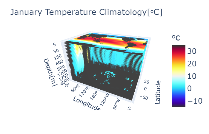
You can see a 3D interactive plot here.

Compute Anomalies

Computing anomalies from this point is simple. Merely subtract each data point with their corresponding climatology:

anom = data - clim

Standardized anomalies are anomalies divided by standard deviation. These are not used in the computation because it will amplify errors due to the nature of the data. This was only added for completeness.

stnd_anom = anom/sdev

To compute weighted anomalies recall the weight:

In python this is:

# lattitude values
x = linspace(0, 360-1, 360)
y = linspace(-90, 90-1, 180)

xx, yy = meshgrid(x, y)
y_temp = yy.flatten()

yy = yy.transpose()
y_temp = yy.flatten()

# area weight for lattitude values
area_w = np.cos(y_temp*math.pi/180)

# area weights for depth
area_weight = []

for i in range(tot_depths):
    if i == 0:
        area_weight.append(np.sqrt(5 * area_w)) # first depth thickness is just 0-5m
    else:
        area_weight.append( np.sqrt((depths[i] - depths[i - 1]) * area_w))
        
# Turning weights into one array
area_weight = np.mat(area_weight)
area_weight = area_weight.flatten()
area_weight = area_weight.T


# Multiply area weight
weighted_A = np.empty((N,Y)) * np.nan # new array of weighted anomalies
weighted_A = np.multiply(anom , area_weight) # multiply weights and anomalies

Compute Covariance, Eigenvectors, and Eigenvalues

Because the data takes into account land, there are NaN values in the data. To get rid of this we take advantage of the fact that no matter what year it is land does not move. As a result if a row has a NaN value every column in that row also has a NaN value meaning that entire row is NaN. This makes it easy to know how many rows have values and how many rows do not have values. We can then fill a new matrix with only values and no NaNs.

Finding how many rows have values:

# find which indicies have data (are not NaN)
numrows = np.argwhere(np.isnan(weighted_A[:,0]) == False)
new_N = round(numrows.shape[0]) # new N dimension without NaNs

Now we create a matrix with only values

new_anom = np.empty((new_N,Y)) * np.nan
for i in range(new_N):
        new_anom[i,:] = weighted_A[numrows[i,0],:]
new_anom = np.mat(new_anom)

Covariance is computed as explained above:

cov = (new_anom.T * new_anom)

The eigenvalues and eigenvectors are found using:

eigvals, eigvecs = np.linalg.eig(cov)

These eigenvalues and eigenvectors ARE NOT sorted. Its easy to sort eigenvalues low to higher values using a python function which keeps track of the correct indexing:

# find correct index
eig_index = np.argsort(eigvals)
eig_index = np.flip(eig_index)

# sort evals
new_eigvals = eigvals[eig_index[:]]
eigvals = new_eigvals

# sort evecs
new_eigvecs = eigvecs[:,eig_index]
eigvecs = new_eigvecs 

The figure below shows both the variance percentage and cumulative variance percentage. You can also download the code to replicate all images from my github.

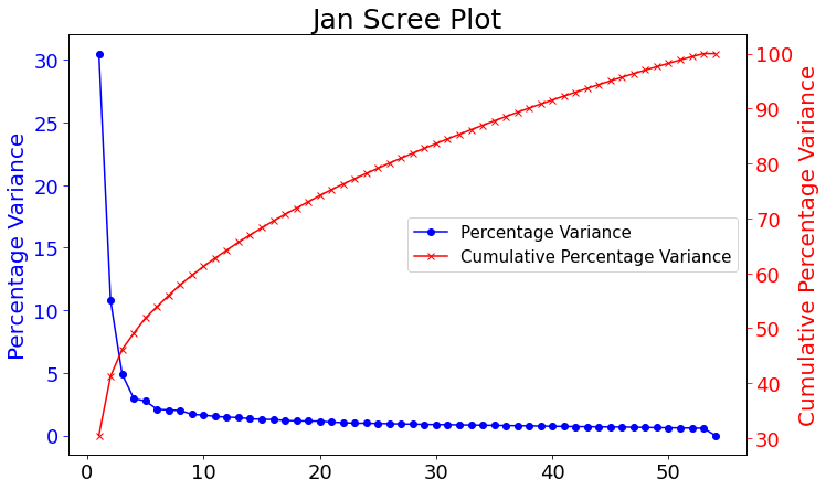
This scree plot shows the percentage variance of each mode and up to how much percentage variance cumulatively we will have at a specific mode. The latter will come in handy during the multivariate regression in telling us how many modes we would want to use for a large percent of information.

Computing 3D EOF using SVD

Using SVD only requires the data to be formatted correctly.

from eofs.standard import Eof
dat = np.array(weighted_A.T) # solver only takes in arrays
solver = Eof(dat) # define solver
eofs = solver.eofs() # compute EOFs 
eofs = eofs.T
eofs = eofs/area_weight[:,0] # get physical EOFs (without weight)

The resulting EOFs are the same as the next section.

Computing 3D EOFs using Temporal Covariance

EOFs are computed by finding the eigenvectors of the temporal covariance matrix, multiplying eigenvectors by the anomalies, and dividing the magnitude of the multiplication.

ev = eigvecs.T
EOFs = []
for j in range(Y):
    EOFs.append(np.matmul(weighted_A , ev[j].T))
    
EOF = np.array(EOFs)
EOF = np.squeeze(EOF)
EOF = EOF.T

We need to divide by the magnitude and need to get rid of NaNs again then divide

# get rid of NaNs
na_rows = np.argwhere(np.isnan(EOF[:,0]) == False) # find which rows have numbers
new_N = round(na_rows.shape[0]) # define new spatial dimension
# fill new matrix with no NaNs
new_EOF = np.empty((numrows.shape[0],Y))*np.nan
for i in range(numrows.shape[0]):
        new_EOF[i,:] = EOF[numrows[i,0],:]
new_EOF = np.mat(new_EOF)

# divide by magnitude to normalize
mag = np.linalg.norm(new_EOF, axis = 0)
for i in range(Y):
    EOF[:,i] = EOF[:,i]/mag[i]

As a way to check that these EOFs are valid the magnitude of each EOF mode should be 1.

# checking magnitude of EOF. If magnitude is not one error will be raised
for col_i in range(54):
    is_one = np.linalg.norm(new_EOF[:,col_i])
    if not np.isclose(is_one, 1):
        raise ValueError(f"EOF {col_i} is not one")

It is also important to check othogonality.

# Check to make sure vectors are orthogonal
n, m = new_EOF.shape
for col_i in range(m):
    for col_j in range(m):
        if col_i < col_j:  # use strictly less than because we don't want to consider a column with itself, and the dot product is commutable so order doesn't matter
            is_orthogonal = np.dot(new_EOF[:, col_i], new_EOF[:, col_j])
            if not np.isclose(is_orthogonal, 0) and col_j != 53:
                pprint(f"EOF Mode {col_i} and EOF Mode {col_j} are not orthogonal.")
                pprint(np.dot(new_EOF[:, col_i], new_EOF[:, col_j]))

finally to find physical EOFs divide by the area weight

EOF = EOF/area_weight[:,0]

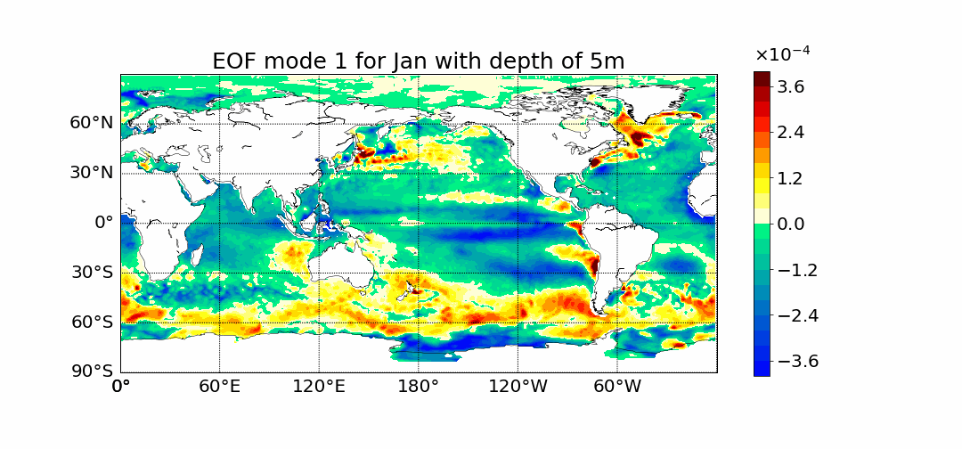
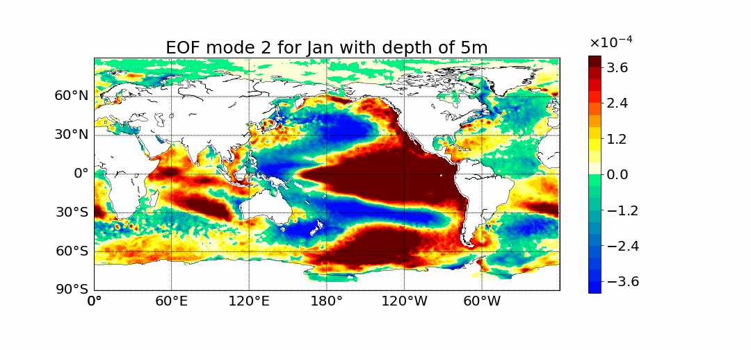
These are the resulting EOFs computed from time covariance.

Surprisingly the first mode does not show the most prominent characteristic to be El Nino. This is what previous calculations done in 2D showed. The first mode has the most amount of percent variance being at around 30%. Meaning most variance is found in the first mode. We would expect then for El Nino to appear within this mode but instead we see equitorial upwelling. This is when deep ocean waters rise up and push surface waters outwards. The next mode starts to show the split between cold and warmer waters at the oceans surface as expected from El Nino.

If you have any further questions please email me at dlafarga9505@sdsu.edu

References

Shen SSP, Somerville RCJ (2019) Climate Mathematics: Theory and Applications. Cambridge University Press

Dawson, A. (2016). eofs: A Library for EOF Analysis of Meteorological, Oceanographic, and Climate Data. Journal of Open Research Software, 4(1), e14. DOI: http://doi.org/10.5334/jors.122

Shen SSP, Behm GP, Song YT, et al (2017) A dynamically consistent reconstruction of ocean temperature. Journal of Atmospheric and Oceanic Technology 34(5):1061 – 1082. https://doi.org/10.1175/JTECH-D-16-0133.1